Nonlocal fundamental splines on rectangular finite elements

N.N.Doniyorov^1,2∗

Abstract

In this work, we investigate the construction of nonlocal fundamental splines on rectangular finite elements. To achieve this, we utilize the coefficients of an optimal algebraic-trigonometric interpolation formula, derived via Sobolev’s method in a Hilbert space of differentiable functions. Furthermore, we establish and prove a theorem that characterizes the essential properties of these nonlocal fundamental splines.

Keywords: Interpolation; optimal interpolation formula; error functional; Hilbert space; approximation; fundamental spline; finite elements.

AMS Subject Classification (2020): Primary: 41A05, 41A15; Secondary: 65D05, 65D07.

1. Introduction

It is known that function interpolation is used in solving many practical problems. In particular, interpolation methods are widely used in modeling complex engineering systems and reconstructing computed tomography images. In interpolation theory, it is of fundamental importance to construct optimal interpolation formulas corresponding to fundamental splines and to evaluate their errors. The problem of constructing an optimal

(^𝑚) interpolation formula was first posed and investigated in 1961 by S. L. Sobolev in the Hilbert space 𝑊₂                       [1].

(^𝑚)

To this end, S. L. Sobolev utilized a discrete analogue 𝐷_ℎ𝐻 (ℎ𝛽) of the polyharmonic differential operator

                                                                                         2            𝜕2                    𝜕2 !𝑚

𝜕

                                                                          Δ^𝑚 =               +            + ... +        .

                                                                                             2            2                     2

                                                                                        𝜕𝑥        𝜕𝑥                  𝜕𝑥

                                                                                             1            2                     𝑛

(^𝑚)

The construction of the discrete operator 𝐷_ℎ𝐻 (ℎ𝛽) in the 𝑛-dimensional case is a very difficult problem. For 𝑛 = 1, the problem of constructing optimal interpolation formulas using S. L. Sobolev’s method has been extensively studied by Kh. M. Shadimetov and A. R. Hayotov [2, 3, 4, 5, 6].

In particular, a discrete analogue Δ₂(^ℎ𝛽) of the differential operator _𝑑𝑥^𝑑6₆ + 2^𝜔2 _𝑑𝑥^𝑑4₄ + ^𝜔4 _𝑑𝑥^𝑑2₂ was constructed anditspropertieswereinvestigatedin[7].Subsequently,in[8],anoptimalalgebraic-trigonometricinterpolation formula was developed by utilizing the results obtained in [7]. In the present work, we construct nonlocal fundamentalsplinesoftwovariablesandinvestigatetheirkeyproperties.Tothisend,weemploythecoefficients of the optimal algebraic-trigonometric interpolation formula established in [8]. For the sake of completeness, a brief overview of these results is presented in the next section.

Received : 01–february–2026, Accepted : 30–may–2026

* Corresponding author

2. An algebraic-trigonometric optimal interpolation formula in the Hilbert space 𝐾(³⁾

2,𝜔

We consider the Hilbert space defined in the form [6]

                                  (_,𝜔3)                                   R ′′                                                               ′′′

                                   𝐾2 = {𝜑 : [0, 1] →         |𝜑   is absolutely continuous and 𝜑      ∈ 𝐿₂(0, 1)} .

This space is equipped by the norm

                                                                                       1                                                  

Suppose we are given the values 𝜑(𝑥₀), 𝜑(𝑥₁), . . . , 𝜑(𝑥_𝑁) of a function 𝜑 at the nodes 𝑥_𝑘 = 𝑘ℎ for 𝑘 = 0, 1, . . . , 𝑁, where ℎ = _𝑁¹ . We consider the problem of approximating the function 𝜑 by an elementary function 𝑃3(𝜑, 𝑥) as follows:

𝜑(𝑥)  𝑃₃(𝜑, 𝑥) for𝑥 ∈ [0, 1],

where

𝑁

∑︁

                                                                                   𝑃₃(𝜑, 𝑥) = 𝐶_𝛽(𝑥)𝜑(𝑥_𝛽)                                                                              (2.1)

𝛽=0

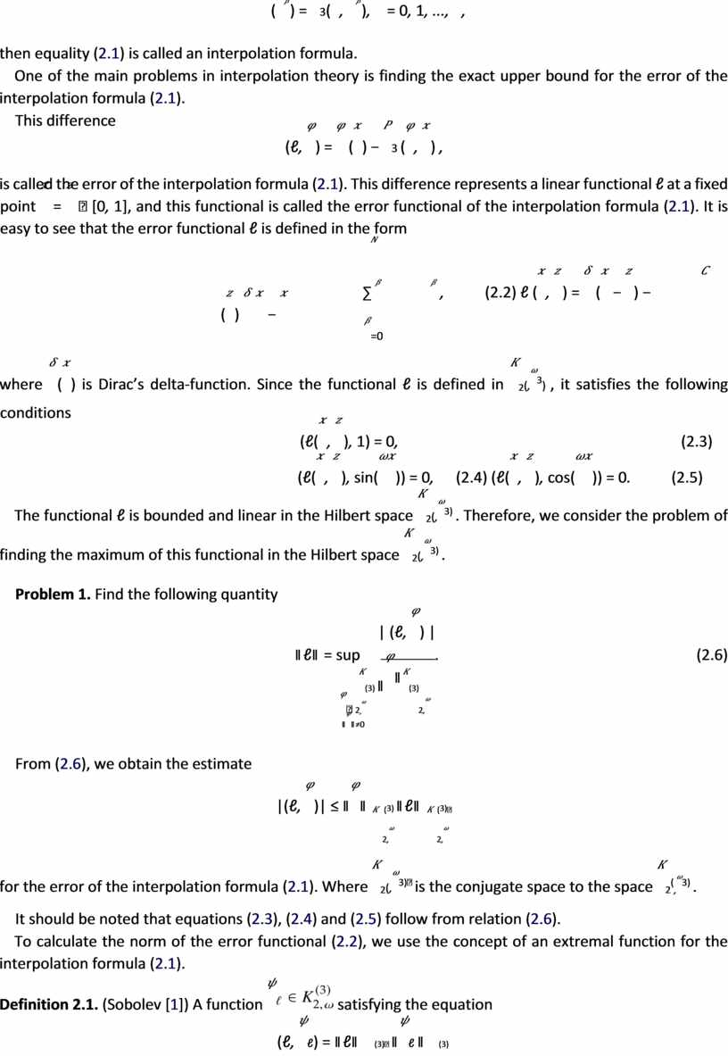
is an approximating function and 𝐶_𝛽 (𝑥) (𝛽 = 0, 1, ..., 𝑁) are its coefficients. If the approximating function 𝑃3(𝜑, 𝑥) satisfies the interpolation conditions

𝜑(𝑥_𝛽) = 𝑃3(𝜑, 𝑥_𝛽), 𝛽 = 0, 1, ..., 𝑁,

then equality (2.1) is called an interpolation formula.

One of the main problems in interpolation theory is finding the exact upper bound for the error of the interpolation formula (2.1).

This difference

(ℓ, 𝜑) = 𝜑 (𝑥) − 𝑃3 (𝜑, 𝑥) ,

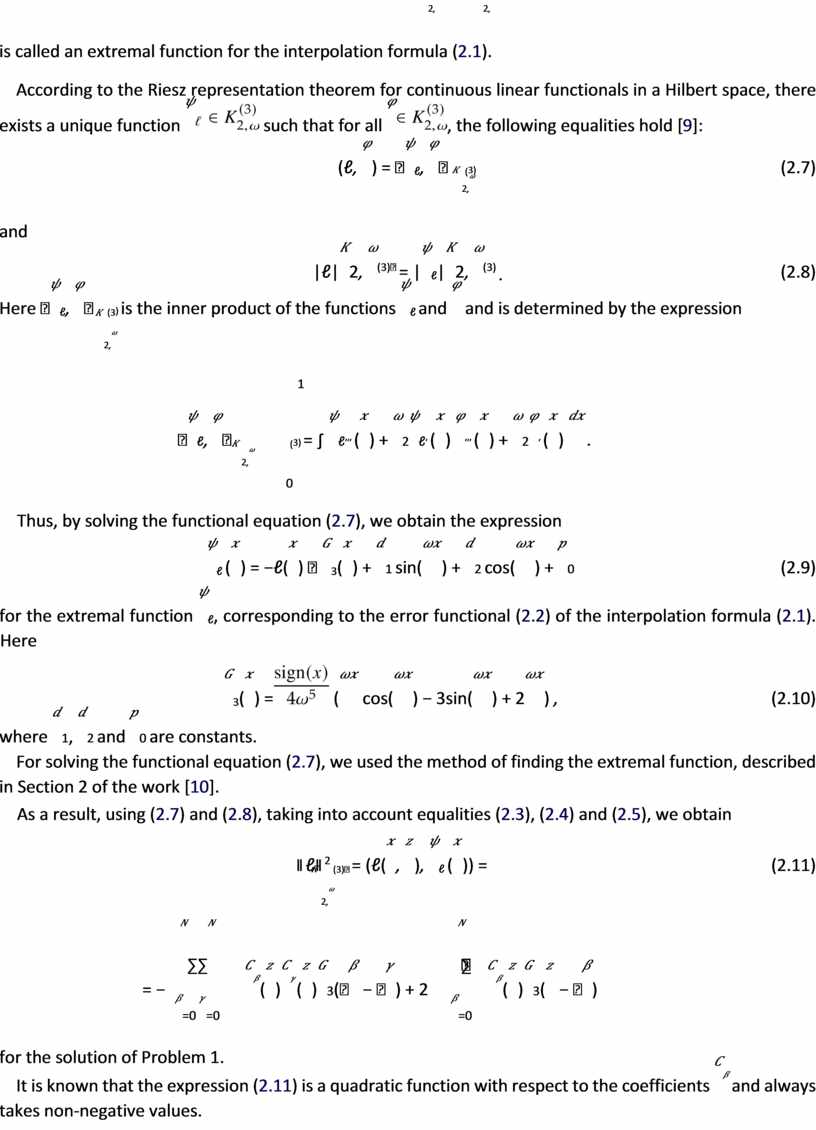
is called the error of the interpolation formula (2.1). This difference represents a linear functional ℓ at a fixed point 𝑥 = 𝑧 ∈ [0, 1], and this functional is called the error functional of the interpolation formula (2.1). It is easy to see that the error functional ℓ is defined in the form

𝑁

∑︁ _{𝛽                      𝛽} ,            (2.2) ℓ (𝑥, 𝑧) = 𝛿 (𝑥 − 𝑧) −              𝐶 (𝑧) 𝛿 𝑥 − 𝑥

𝛽=0

where 𝛿(𝑥) is Dirac’s delta-function. Since the functional ℓ is defined in 𝐾₂(,𝜔³) , it satisfies the following conditions

                                                                                        (ℓ(𝑥, 𝑧), 1) = 0,                                                                                  (2.3)

(ℓ(𝑥, 𝑧), sin(𝜔𝑥)) = 0,      (2.4) (ℓ(𝑥, 𝑧), cos(𝜔𝑥)) = 0.           (2.5)

The functional ℓ is bounded and linear in the Hilbert space 𝐾₂(,𝜔³⁾ . Therefore, we consider the problem of finding the maximum of this functional in the Hilbert space 𝐾₂(,𝜔³⁾ .

Problem 1. Find the following quantity

| (ℓ, 𝜑) |

                                                                                      ∥ℓ∥ = sup      .                                                                           (2.6)

𝐾(3) ∥^𝜑∥𝐾(3)

                                                                                                   𝜑∈ 2_,𝜔                        2,𝜔

∥𝜑∥≠0

From (2.6), we obtain the estimate

                                                                                 |(ℓ, 𝜑)| ≤ ∥𝜑∥     ₍3) ∥ℓ∥    ₍3)_∗

                                                                                                             𝐾              𝐾

                                                                                                                2,𝜔                   2,𝜔

for the error of the interpolation formula (2.1). Where 𝐾₂(,𝜔^3)∗ is the conjugate space to the space 𝐾₂⁽_,𝜔³⁾ .

It should be noted that equations (2.3), (2.4) and (2.5) follow from relation (2.6).

To calculate the norm of the error functional (2.2), we use the concept of an extremal function for the interpolation formula (2.1).

Definition 2.1. (Sobolev [1]) A function 𝜓 satisfying the equation

                                                                                 (ℓ, 𝜓ℓ) = ∥ℓ∥    (3)∗ ∥𝜓ℓ ∥    (3)

𝐾 𝐾 2,𝜔                 2,𝜔

is called an extremal function for the interpolation formula (2.1).

According to the Riesz representation theorem for continuous linear functionals in a Hilbert space, there exists a unique function 𝜓 such that for all 𝜑, the following equalities hold [9]:

                                                                                        (ℓ, 𝜑) = ⟨𝜓_ℓ, 𝜑⟩     ₍3)                                                                                                                       (2.7)

𝐾 2,𝜔

and

                                                                                  |ℓ|𝐾2, 𝜔^(3)∗ = |𝜓_ℓ|𝐾2, 𝜔⁽³⁾ _.                                                                        (2.8)

Here ⟨𝜓_ℓ, 𝜑⟩   ₍₃) is the inner product of the functions 𝜓_ℓ and 𝜑 and is determined by the expression

𝐾

2,𝜔

1

                                              ⟨𝜓ℓ, 𝜑⟩               ₍3) = ∫ 𝜓ℓ′′′ (𝑥) + 𝜔2𝜓ℓ′ (𝑥) 𝜑′′′ (𝑥) + 𝜔2𝜑′ (𝑥) 𝑑𝑥.

𝐾 2,𝜔

0

Thus, by solving the functional equation (2.7), we obtain the expression

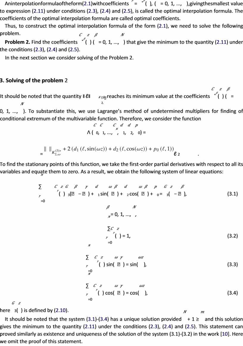
                                                      𝜓_ℓ (𝑥) = −ℓ(𝑥) ∗ 𝐺₃(𝑥) + 𝑑1 sin(𝜔𝑥) + 𝑑2 cos(𝜔𝑥) + 𝑝0                                                      (2.9)

for the extremal function 𝜓_ℓ, corresponding to the error functional (2.2) of the interpolation formula (2.1). Here

                                                          𝐺₃(𝑥) = (𝜔𝑥 cos(𝜔𝑥) − 3sin(𝜔𝑥) + 2𝜔𝑥) ,                                                       (2.10)

where 𝑑1, 𝑑2 and 𝑝0 are constants.

For solving the functional equation (2.7), we used the method of finding the extremal function, described in Section 2 of the work [10].

As a result, using (2.7) and (2.8), taking into account equalities (2.3), (2.4) and (2.5), we obtain

                                                                             ∥ℓ∥² _(3)∗ = (ℓ(𝑥, 𝑧), 𝜓_ℓ (𝑥)) =                                                                          (2.11)

𝐾

2,𝜔

                                               𝑁      𝑁                                                               𝑁

                                                 ∑︁∑︁                                                                 ∑︁

                                     = −                     𝐶_𝛽(𝑧)𝐶_𝛾(𝑧)𝐺3(ℎ𝛽 − ℎ𝛾) + 2               𝐶_𝛽(𝑧)𝐺3(𝑧 − ℎ𝛽)

                                              𝛽=0 𝛾=0                                                            𝛽=0

for the solution of Problem 1.

It is known that the expression (2.11) is a quadratic function with respect to the coefficients 𝐶_𝛽 and always takes non-negative values.

Aninterpolationformulaoftheform(2.1)withcoefficients𝐶_𝛽 = 𝐶˚_𝛽(𝑧), (𝛽 = 0, 1, ..., 𝑁),givingthesmallest value to expression (2.11) under conditions (2.3), (2.4) and (2.5), is called the optimal interpolation formula. The coefficients of the optimal interpolation formula are called optimal coefficients.

Thus, to construct the optimal interpolation formula of the form (2.1), we need to solve the following problem.

Problem 2. Find the coefficients 𝐶˚_𝛽(𝑧) (𝛽 = 0, 1, ..., 𝑁) that give the minimum to the quantity (2.11) under the conditions (2.3), (2.4) and (2.5).

In the next section we consider solving of the Problem 2.

3. Solving of the problem 2

It should be noted that the quantity ∥ℓ∥        ₍₃)_∗ reaches its minimum value at the coefficients 𝐶˚_𝛽(𝑧) (𝛽 =

𝐾 2, 𝜔

0, 1, ..., 𝑁). To substantiate this, we use Lagrange’s method of undetermined multipliers for finding of conditional extremum of the multivariable function. Therefore, we consider the function

Λ (𝐶0,𝐶1, ...,𝐶_𝑁, 𝑑1, 𝑑2, 𝑝0) =

                                   = ℓ 2               .

To find the stationary points of this function, we take the first-order partial derivatives with respect to all its variables and equate them to zero. As a result, we obtain the following system of linear equations:

𝑁

∑︁

                                               𝐶_𝛾(𝑧)𝐺₃(ℎ𝛽 − ℎ𝛾) + 𝑑₁ sin(𝜔ℎ𝛽) + 𝑑₂ cos(𝜔ℎ𝛽) + 𝑝₀ = 𝐺₃(𝑧 − ℎ𝛽),                                   (3.1)

𝛾=0

𝛽 = 0, 1, ..., 𝑁,

𝑁

∑︁

                                                                                                𝐶_𝛾(𝑧) = 1,                                                                                    (3.2)

𝛾=0

𝑁

∑︁

                                                                                  𝐶_𝛾(𝑧) sin(𝜔ℎ𝛾) = sin(𝜔𝑧),                                                                      (3.3)

𝛾=0

𝑁

∑︁

                                                                                 𝐶_𝛾(𝑧) cos(𝜔ℎ𝛾) = cos(𝜔𝑧),                                                                     (3.4)

𝛾=0

here 𝐺3(𝑧) is defined by (2.10).

It should be noted that the system (3.1)-(3.4) has a unique solution provided 𝑁 + 1 ≥ 𝑚 and this solution gives the minimum to the quantity (2.11) under the conditions (2.3), (2.4) and (2.5). This statement can proved similarly as existence and uniqueness of the solution of the system (3.1)-(3.2) in the work [10]. Here we omit the proof of this statement.

To find the analytical solution the system of linear equations (3.1)-(3.3), we use the discrete analog 𝐷3(ℎ𝛽) of the differential operator _𝑑𝑥^𝑑6₆ + 2𝜔² _𝑑𝑥^𝑑4₄ + 𝜔⁴ _𝑑𝑥^𝑑2₂ and the properties of this discrete analog. For this purpose, we present the following theorems.

𝐷₃ (ℎ𝛽) ∗ sin (𝜔ℎ𝛽) = 0,

𝐷₃ (ℎ𝛽) ∗ cos (𝜔ℎ𝛽) = 0,

𝐷₃ (ℎ𝛽) ∗ (𝜔ℎ𝛽) sin (𝜔ℎ𝛽) = 0,

𝐷₃ (ℎ𝛽) ∗ (𝜔ℎ𝛽) cos (𝜔ℎ𝛽) = 0,

𝐷₃ (ℎ𝛽) ∗ 1 = 0,

𝐷₃ (ℎ𝛽) ∗ (𝜔ℎ𝛽) = 0.

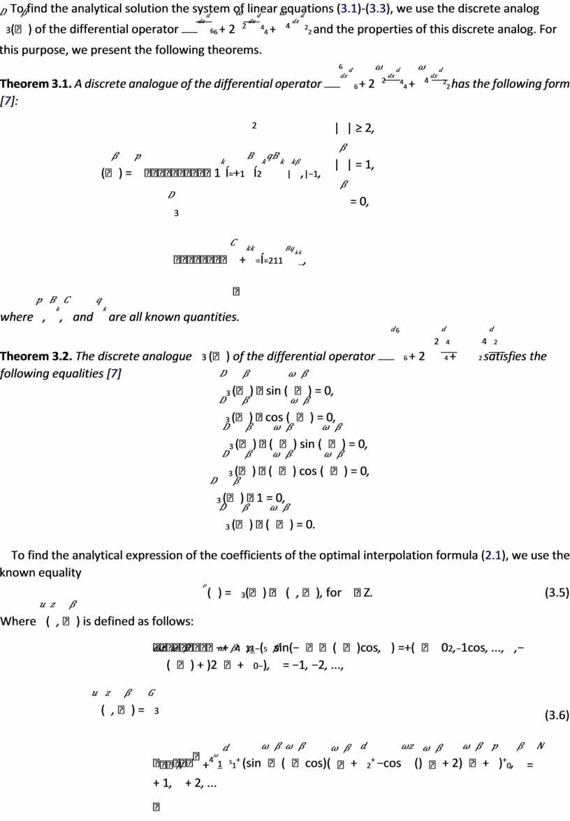
To find the analytical expression of the coefficients of the optimal interpolation formula (2.1), we use the known equality



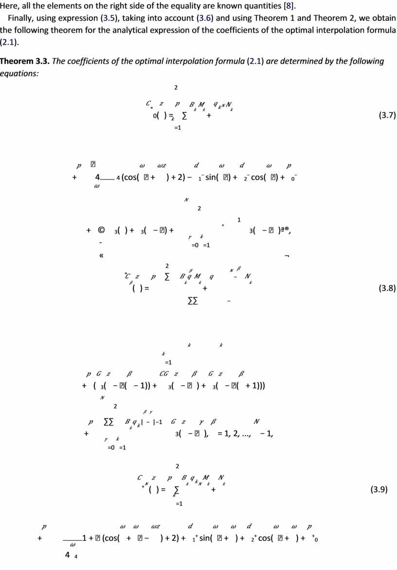
Here, all the elements on the right side of the equality are known quantities [8].

Finally, using expression (3.5), taking into account (3.6) and using Theorem 1 and Theorem 2, we obtain the following theorem for the analytical expression of the coefficients of the optimal interpolation formula (2.1).

Theorem 3.3. The coefficients of the optimal interpolation formula (2.1) are determined by the following equations:

2

                                                                              𝐶^˚0(𝑧) = 𝑝 ∑︁ _{𝐵𝑘 𝑀𝑘} + 𝑞𝑘^𝑁 _𝑁𝑘                                                                              (3.7)

𝑘=1

                                                 _ℎ                                                                                                                

                                       +𝑝      4 4 (cos(𝜔ℎ + 𝜔𝑧) + 2) − 𝑑₁⁻ sin(𝜔ℎ) + 𝑑₂⁻ cos(𝜔ℎ) + 𝑝₀⁻

_𝜔

                                                                                                   𝑁     2

                                                                                                     ∑︁∑︁                −

                                                                                                     𝑘               𝑘

𝑘=1

+𝑝 (𝐺₃(𝑧 − ℎ(𝛽 − 1)) + 𝐶𝐺₃(𝑧 − ℎ𝛽) + 𝐺₃(𝑧 − ℎ(𝛽 + 1)))

                                                      𝑁     2

                                                        ∑︁∑︁              |^𝛽−^𝛾|−1

                                             +𝑝                 𝐵_𝑘𝑞𝑘                𝐺3(𝑧 − ℎ𝛾), 𝛽 = 1, 2, ..., 𝑁 − 1,

𝛾=0 𝑘=1

2

                                                                          𝐶˚_𝑁 (𝑧) = 𝑝 ∑︁ 𝐵_𝑘 𝑞𝑘_𝑁 𝑀_𝑘 + 𝑁_𝑘                                                                             (3.9)

𝑘=1

                    +𝑝        1 + ℎ (cos(𝜔 + 𝜔ℎ − 𝜔𝑧) + 2) + 𝑑₁⁺ sin(𝜔ℎ + 𝜔) + 𝑑₂⁺ cos(𝜔ℎ + 𝜔) + 𝑝⁺₀

4_𝜔4

                                                                                                        𝑁     2

                                                                                                         ∑︁∑︁               ^{𝑁 −𝛾−1}

+𝑝 ©𝐶𝐺₃(𝑧 ⁻ 1) + 𝐺₃(𝑧 ⁻ 1 + ℎ) +             _𝐵𝑘𝑞𝑘       _𝐺3(𝑧 − ℎ𝛾)ª®, ­

𝛾=0 𝑘=1

                                      «                                                                                                                      ¬

here, all the elements on the right side of the equalities are known quantities [8].

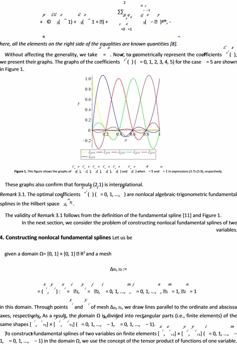
Without affecting the generality, we take 𝑧 = 𝑥. Now, to geometrically represent the coefficients 𝐶˚_𝑖(𝑥), we present their graphs. The graphs of the coefficients 𝐶˚_𝑖(𝑥) (𝑖 = 0, 1, 2, 3, 4, 5) for the case 𝑁 = 5 are shown in Figure 1.

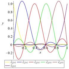
Figure 1. This figure shows the graphs of 𝐶^˚₀(𝑥), 𝐶^˚₁(𝑥), 𝐶^˚₂(𝑥), 𝐶^˚₃(𝑥), 𝐶^˚₄(𝑥) and 𝐶^˚₅(𝑥) when 𝑁 = 5 and 𝜔 = 1 in expressions (3.7)-(3.9), respectively.

These graphs also confirm that formula (2.1) is interpolational.

Remark 3.1. The optimal coefficients 𝐶˚_𝑖(𝑥) (𝑖 = 0, 1, ..., 𝑁) are nonlocal algebraic-trigonometric fundamental splines in the Hilbert space 𝐾₂(,𝜔³⁾ .

The validity of Remark 3.1 follows from the definition of the fundamental spline [11] and Figure 1.

In the next section, we consider the problem of constructing nonlocal fundamental splines of two variables.

4. Constructing nonlocal fundamental splines Let us be given a domain Ω= [0, 1] × [0, 1] ⊂ R² and a mesh

Δℎ1, ℎ2 :=

= (𝑥_𝑖, 𝑦 _𝑗) : 𝑥_𝑖 = 𝑖ℎ1, 𝑦 _𝑗 = 𝑗ℎ2, 𝑖 = 0, 1, ..., 𝑚, 𝑗 = 0, 1, ..., 𝑛, ℎ1𝑚 = 1, ℎ2𝑛 = 1

in this domain. Through points 𝑥_𝑖 and 𝑦 _𝑗 of mesh Δ_ℎ1, ℎ₂, we draw lines parallel to the ordinate and abscissa axes, respectively. As a result, the domain Ω is divided into rectangular parts (i.e., finite elements) of the same shapes [𝑥_𝑖, 𝑥_𝑖+₁] × [𝑦 _𝑗, 𝑦 _𝑗+₁] (𝑖 = 0, 1, ..., 𝑚 − 1, 𝑗 = 0, 1, ..., 𝑛 − 1).

To construct fundamental splines of two variables on finite elements [𝑥_𝑖, 𝑥_𝑖+1] × [𝑦 _𝑗, 𝑦 _𝑗+1] (𝑖 = 0, 1, ..., 𝑚 − 1, 𝑗 = 0, 1, ..., 𝑛 − 1) in the domain Ω, we use the concept of the tensor product of functions of one variable.

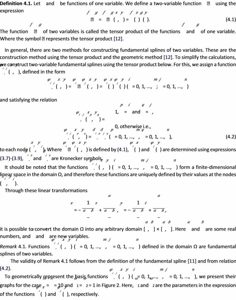
Definition 4.1. Let 𝑓 and 𝑔 be functions of one variable. We define a two-variable function 𝑓 ⊗ 𝑔 using the expression

                                                                              𝑓 ⊗ 𝑔 = 𝑓 ⊗ 𝑔(𝑥, 𝑦) = 𝑓 (𝑥)𝑔(𝑦).                                                                    (4.1)

The function 𝑓 ⊗ 𝑔 of two variables is called the tensor product of the functions 𝑓 and 𝑔 of one variable. Where the symbol ⊗ represents the tensor product [12].

In general, there are two methods for constructing fundamental splines of two variables. These are the construction method using the tensor product and the geometric method [12]. To simplify the calculations, we construct two-variable fundamental splines using the tensor product below. For this, we assign a function

𝜑_{𝑖, 𝑗} (𝑥, 𝑦), defined in the form

𝜑_{𝑖, 𝑗} (𝑥, 𝑦) = 𝜑_𝑖 ⊗ 𝜑_𝑗 (𝑥, 𝑦) = 𝜑_𝑖(𝑥)𝜑_𝑗 (𝑦) (𝑖 = 0, 1, ..., 𝑚; 𝑗 = 0, 1, ..., 𝑛)

and satisfying the relation

 1, 𝑝 = 𝑖 and 𝑞 = 𝑗,

𝜑𝑖, 𝑗 (𝑥𝑝, 𝑦𝑞) =

0, otherwise i.e.,

                                                         𝜑_{𝑖, 𝑗} (𝑥_𝑝, 𝑦_𝑞) = 𝛿_{𝑖, 𝑝}𝛿_{𝑗, 𝑞} (𝑝 = 0, 1, ..., 𝑚, 𝑞 = 0, 1, ..., 𝑛),                                                (4.2)

to each node (𝑥_𝑖, 𝑦 _𝑗). Where 𝜑_𝑖 ⊗ 𝜑_𝑗 (𝑥, 𝑦) is defined by (4.1), 𝜑_𝑖(𝑥) and 𝜑_𝑗 (𝑦) are determined using expressions (3.7)-(3.9), 𝛿_{𝑖, 𝑝} and 𝛿_{𝑗, 𝑞} are Kronecker symbols.

It should be noted that the functions 𝜑_{𝑖, 𝑗} (𝑥, 𝑦) (𝑖 = 0, 1, ..., 𝑚, 𝑗 = 0, 1, ..., 𝑛) form a finite-dimensional linear space in the domain Ω, and therefore these functions are uniquely defined by their values at the nodes

(𝑥𝑖, 𝑦 𝑗).

Through these linear transformations

                                                                              1                 𝑎                        1                𝑎

                                                               𝑥 = −             𝑠 +              , 𝑦 = −             𝑡 +            ,

                                                                           𝑎 − 𝑏         𝑎 − 𝑏                𝑎 − 𝑏         𝑎 − 𝑏

it is possible to convert the domain Ω into any arbitrary domain [𝑎, 𝑏] × [𝑎, 𝑏]. Here 𝑎 and 𝑏 are some real numbers, and 𝑠 and 𝑡 are new variables.

Remark 4.1. Functions 𝜑_{𝑖, 𝑗} (𝑥, 𝑦) (𝑖 = 0, 1, ..., 𝑚, 𝑗 = 0, 1, ..., 𝑛) defined in the domain Ω are fundamental splines of two variables.

The validity of Remark 4.1 follows from the definition of the fundamental spline [11] and from relation

(4.2).

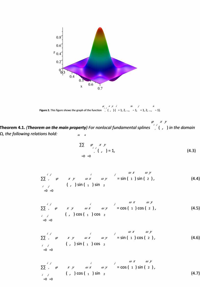
To geometrically represent the basis functions 𝜑_{𝑖, 𝑗} (𝑥, 𝑦) (𝑖 = 0, 1, ..., 𝑚, 𝑗 = 0, 1, ..., 𝑛), we present their graphs for the case 𝑚 = 𝑛 = 10 and 𝜔1 = 𝜔2 = 1 in Figure 2. Here, 𝜔1 and 𝜔2 are the parameters in the expression of the functions 𝜑_𝑖(𝑥) and 𝜑_𝑗 (𝑦), respectively.

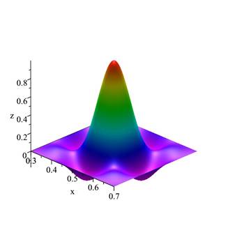
Figure 2. This figure shows the graph of the function 𝜑_{𝑖, 𝑗} (𝑥, 𝑦) (𝑖 = 1, 2, ..., 𝑚 − 1, 𝑗 = 1, 2, ..., 𝑛 − 1).

Theorem 4.1. (Theorem on the main property) For nonlocal fundamental splines 𝜑_{𝑖, 𝑗} (𝑥, 𝑦) in the domain Ω, the following relations hold:

                                                                                   𝑚     𝑛

∑︁∑︁

                                                                                                𝜑_{𝑖, 𝑗} (𝑥, 𝑦) = 1,                                                                            (4.3)

𝑖=0 𝑗=0

where 𝜔1 and 𝜔2 are elements of the set R \ {0}.

The proof of Theorem 4.1 follows from Definition 4.1 and from equalities (2.3), (2.4) and (2.5).

From relations (4.3)-(4.7), it can be stated that the nonlocal fundamental splines 𝜑_{𝑖, 𝑗} (𝑥, 𝑦) (𝑖 = 0, 1, ..., 𝑚, 𝑗 = 0, 1, ..., 𝑛)            accurately           reconstruct        any        linear    combination      of           the         functions             1, sin(𝜔1𝑥) sin(𝜔2𝑦), cos(𝜔1𝑥) cos(𝜔2𝑦), sin(𝜔1𝑥) cos(𝜔2𝑦) and cos(𝜔1𝑥) sin(𝜔2𝑦).

It should be noted that nonlocal fundamental splines 𝜑_{𝑖, 𝑗} (𝑥, 𝑦) (𝑖 = 0, 1, ..., 𝑚, 𝑗 = 0, 1, ..., 𝑛) can be applied to finite element methods and signal processing.

5. Conclusion

In this article, a bounded region on a plane is divided into rectangular finite elements, and nonlocal fundamental splines are constructed on these finite elements. For this, the coefficients of the algebraictrigonometric optimal interpolation formula constructed in the Hilbert space were used. Also, the theorem expressing the main property of these fundamental splines was proven.

Acknowledgements

The author would like to express his deep gratitude to Professor Abdullo R. Hayotov for his valuable feedback and for discussing the results of this research.

References

[1]       Sobolev S.L. Introduction to the Theory of Cubature Formulas (in Russian). Moscow, Nauka, 1974.

                                                                                                      ^𝑚                               (^𝑚)

[2]       Cabada A., Hayotov A.R., Shadimetov Kh.M. Construction of 𝐷 -splines in 𝐿2 (0, 1) space by Sobolev method. Applied Mathematics and Computation, vol. 244, 2014. Pp. 542-551. https://doi.org/10.1016/j.amc.2014.07.033

[3]       Hayotov A.R., Milovanovi𝑐´ G.V., Shadimetov Kh.M. Interpolation splines minimizing a semi-norm. Calcolo, vol.51, 2014. Pp. 245-260.

https://doi.org/10.1007/s10092-013-0080-x

[4]       Shadimetov Kh.M., Hayotov A.R. Construction of interpolation splines minimizing semi-norm in 𝑊2(^𝑚,𝑚−¹⁾ (0, 1) space. Bit Numer. Math., vol.53, 2013. Pp.545-563. https://doi.org/10.1007/s10543-012-0407-z

(^𝑚)

[5]       Shadimetov Kh.M., Hayotov A.R., Nuraliev F.A. Optimal interpolation formulas with derivative in the space 𝐿2 (0, 1). Filomat, vol.33(17), 2019. Pp.5661-5675. https://doi.org/10.2298/FIL1917661S

[6]       Hayotov A.R. Construction of interpolation splines minimizing the semi-norm in the space 𝐾₂ (𝑃_𝑚). Journal of Siberian Federal University.

Mathematics and Physics, vol.11(3), 2018. Pp.383 - 396. https://doi.org/10.17516/1997-1397-2018-11-3-383-396

[7]       Hayotov A.R. Discrete analogs of some differential operators (in Russian). Uzbek Mathematical Journal, no.1, 2012. Pp.151-155.

[8]       Doniyorov N.N. Algebro-trigonometric optimal interpolation formula in a Hilbert space. Problems of computational and applied mathematics, no. 3/1 (50), 2023. Pp. 5-19.

[9]       Kendal Atkinson, Weimin Han. Theoretical Numerical Analysis. Springer Science, Business Media, LLC 2009.

[10]    Hayotov A.R., Milovanović G.V., Shadimetov Kh. M. Optimal quadratures in the sense of Sard in a Hilbert space. Applied Mathematics and Computation, vol.259, 2015. Pp.637-659, https://doi.org/10.1016/j.amc.2015.02.093.

[11]    Zavyalov Yu.S., Kvasov B.I., Miroshnichenko V.L. Methods of spline functions (in Russian). Moscow, Nauka, 1980.

[12]    Zhilin L., Zhonghua Q., Tao T. Numerical Solution of Differential Equations.. Cambridge University Press, 2018.

Affiliations

Doniyorov N.N.

Address: ¹ Asia International University, 74, Gijduvon str., Bukhara 200114, Uzbekistan; ² Bukhara State University, 11, Muhammad Ikbal St., Bukhara, 200114, Uzbekistan. e-mail: doniyorovnn@mail.ru

ORCID ID: https://orcid.org/0009-0001-3889-1641