Поделиться

![]()
AUTONOMOUS EDUCATIONAL ORGANIZATION
«NAZARBAYEV INTELLECTUAL SCHOOLS»
MATHEMATICS IN TALDYKORGAN
NAZARBAYEV INTELLECTUAL SCHOOL OF PHYSICS AND
Practical and laboratory work
11th grade
Level A and AS

![]()
Explanatory note
This manual is intended for teachers and students of Nazarbayev Intellectual Schools. The materials of the collection are focused on the development of the following practical skills of students:
Ø Calculation of errors
Ø Plotting a graph
Ø Determination of the error by the graphical method
Ø Selecting the scale when plotting a graph
Ø Plotting the Best match line
Ø Writing numbers with a certain number of significant digits to a table
Ø Calculation of the average data value
Ø Analysis of error sources
Ø Planning to improve the quality of the experiment
Some practical work is of an alternative nature, i.e. there is data on the experiment. This type of work is aimed at developing data processing skills. The manual provides assessment criteria or mark schemes that can be provided to students for self-and mutual verification. This method of assessment forms students ' understanding of the structure of answers, replenishes the vocabulary of subject terminology.
This collection fully meets the requirements and level of NICHE programs, using these practical and laboratory works, teachers will be able to most effectively explain the material and help students achieve the following educational goals:
Ø Investigation of dependency of ball velocity on its radius at motion in a viscous fluid
Ø Describe an experiment to determine the Young modulus of a metal in the form of a wire;
Ø Investigation of mathematical pendulum oscillations.
Ø Investigate the motion of an oscillator using experimental and graphical methods;
Ø Investigation of spring pendulum oscillations.
Ø Investigation of isothermal process.
Ø Investigation of isobaric process
Ø Determination of water surface tension coefficient
Laboratory work No. 1
Viscosity an experimental exercise Does size matter?
![]() If
the particles are falling in the viscous fluid by their own weight due to gravity, then a terminal velocity, also known as the
settling velocity, is reached when this frictional force combined with the buoyant force exactly balance the gravitational force. The resulting
settling velocity (or terminal velocity) is given by:
If
the particles are falling in the viscous fluid by their own weight due to gravity, then a terminal velocity, also known as the
settling velocity, is reached when this frictional force combined with the buoyant force exactly balance the gravitational force. The resulting
settling velocity (or terminal velocity) is given by:
where:
• vs is the particles' settling velocity (m/s) (vertically
downwards if ρp > ρf, upwards if ρp < ρf), R is the radius of the spherical object (in m)
• g is the gravitational acceleration (m/s2),
• ρp is the mass density of the particles (kg/m3), and ρf is the mass density of the fluid (kg/m3).
• µ is the dynamic (absolute) viscosity (N s/m2),
Stokes' law makes the following assumptions for the behavior of a particle in a fluid:
• Laminar Flow
• Spherical particles
• Homogeneous (uniform in composition) material
• Smooth surfaces
• Particles do not interfere with each other.
Learning Objectives:
1. Know that viscosity is a property of fluids that contributes to ‘frictional drag’, Fd.
2. Measure the settling velocity of different sized clay spheres and graph results LO: “show an understanding of the distinction between systematic errors
(including zero errors) and random errors)”
3. Understand how to calculate viscosity from graphical analysis of gradient.
LO: “derive a relationship between two variables or recognize a constant”
4. .Be able to use experimental data to calculate constants using graphical methods.
LO: “calculate uncertainties (including graphically)” Key Words:
|
English |
Kazakh |
Russian |
|
Velocity |
|
|
|
Density |
|
|
|
Sphere |
|
|
|
Homogeneous |
|
|
Particle
Laminar Flow
Name___________________________________________________grade______________
Tasks:
1. Carry out the experiment to gather data relating spherical radius and settling velocity. Method:
Equipment: Large measuring cylinder – at least 30 cm high, Modeling clay, Viscous liquid, Stopwatch, Ruler
|
|
|
|
Measuring cylinder |
Modeling clay balls |
 Stop watch
What to do:
1. Put viscous liquid into measuring cylinder. Put a mark 5cm below the top level of the liquid and a mark 5cm above the bottom. Measure the distance between the two marks and record:___________________________
2. Make 5 spherical balls from the modeling clay, of different sizes, and measure the diameter using Vernier calipers. Record the radius, R, of each ball and record. Ensure balls fit comfortably into the cylinder. (Make up a suitable table to record all measurements with uncertainties)
3. Allow each ball to drop through the liquid, recording the time it takes to fall between the marks. Record the times. Repeat three times for each ball and average the results.
4. Calculate the settling velocity, v, of each ball.
Analysis
1. Graph ‘v’ versus ‘R’ on a suitable graph paper with ‘error bars’.
2. What is the shape of the graph?
_______________________________________________________________________
3. What is the relationship between ‘v’ and ‘R’?
_______________________________________________________________________
4. Draw another graph of ‘v’ versus ‘R2’ on a suitable graph paper with ‘error bars’
5. What is the shape of this graph?
_
6. Calculate the gradient of the line.
______________________ _
7. Write the equation for the line.
_________________ _
8. Calculate the density of the balls and the viscous fluid.
____ _
______________________________________________________________________
___________________ __
9. Use the gradient and Stokes Law equation to calculate the dynamic viscosity of the fluid.
________________________________________________________________
________________________________________________________________
_________________________________ ___
________________________ ________
________________________________________________________________
10. Write a conclusion and evaluation for this experiment.
______________________________________________________________________________
__________________________________________________________________________
__________________________________________________________________________
______________________________________________________________________________
___
______________________________________________________________________________
__
______________________________________________________________________________
___
______________________________________________________________________________
___

Laboratory work No. 2
Determination of Young's modulus
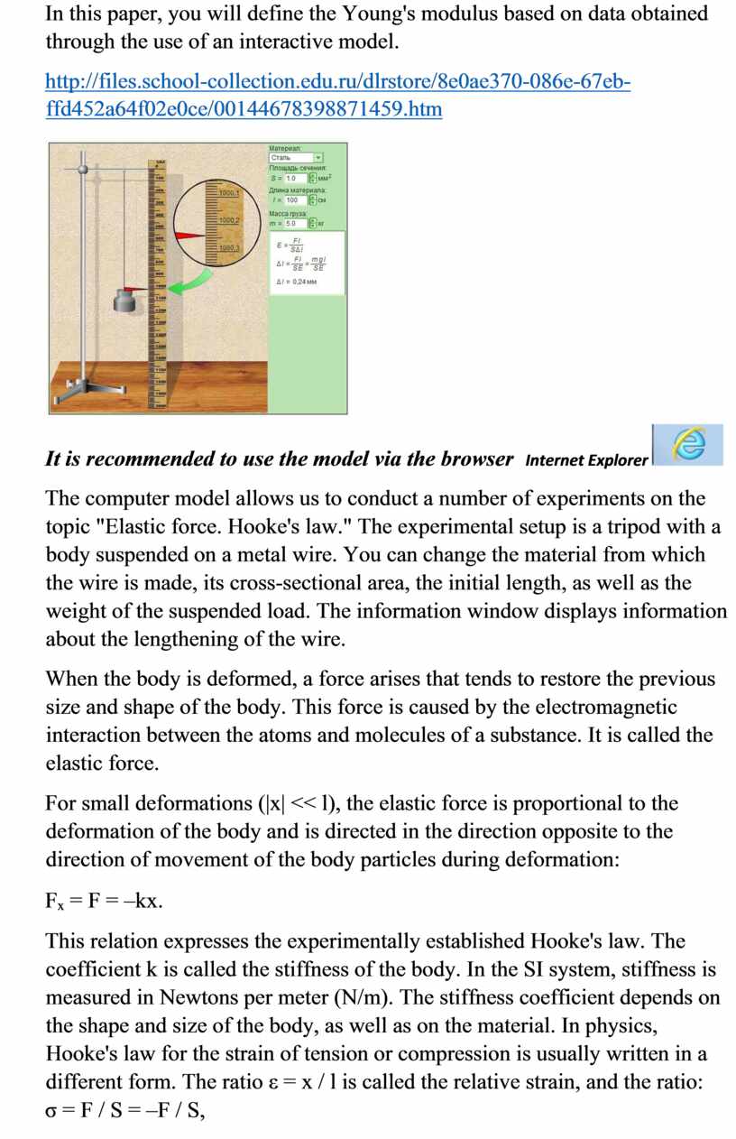
In this paper, you will define the Young's modulus based on data obtained through the use of an interactive model.
http://files.school-collection.edu.ru/dlrstore/8e0ae370-086e-67eb-ffd452a64f02e0ce/00144678398871459.htm

The computer model allows us to conduct a number of experiments on the topic "Elastic force. Hooke's law." The experimental setup is a tripod with a body suspended on a metal wire. You can change the material from which the wire is made, its cross-sectional area, the initial length, as well as the weight of the suspended load. The information window displays information about the lengthening of the wire.
When the body is deformed, a force arises that tends to restore the previous size and shape of the body. This force is caused by the electromagnetic interaction between the atoms and molecules of a substance. It is called the elastic force.
For small deformations (|x| << l), the elastic force is proportional to the deformation of the body and is directed in the direction opposite to the direction of movement of the body particles during deformation:
Fx = F = –kx.
This relation expresses the experimentally established Hooke's law. The coefficient k is called the stiffness of the body. In the SI system, stiffness is measured in Newtons per meter (N/m). The stiffness coefficient depends on the shape and size of the body, as well as on the material. In physics, Hooke's law for the strain of tension or compression is usually written in a different form. The ratio ε = x / l is called the relative strain, and the ratio:
σ = F / S = –F / S,
where S is the cross-sectional area of the deformed body, called the stress. Then
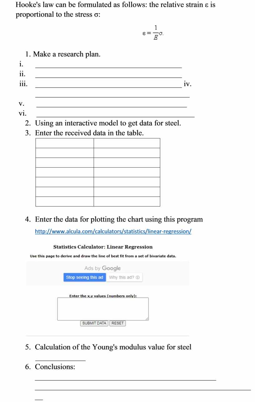
Hooke's law can be formulated as follows: the relative strain ε is proportional to the stress σ:

1. Make a research plan.
i. ______________________________________
ii. ______________________________________
iii. ______________________________________ iv. ________________________________________
v. _______________________________________
vi. _________________________________________
2. Using an interactive model to get data for steel.
3. Enter the received data in the table.
|
|
|
|
|
|
|
|
|
|
|
|
|
|
|
|
|
|
|
|
|
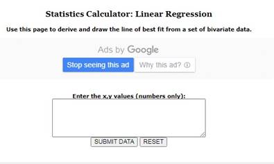
4. Enter the data for plotting the chart using this program
http://www.alcula.com/calculators/statistics/linear-regression/
5. Сalculation of the Young's modulus value for steel
_____________
6. Conclusions: _______________________________________________ __________________________________________________________
__________________________________________________________
Job evaluation criteria:
ü The actions of the plan are consistent and justified
ü All steps are specified until the desired value is obtained
ü Competent wording with the use of terminology on the topic
ü At least 9 readings were selected
ü The graph is built through the use of an interactive application
ü All experimental data are presented in the corresponding values
ü The gradient from the formula is correctly expressed
ü The correct values of the Young's modulus for steel are obtained based on data analysis
Laboratory work No. 3
It is recommended that you spend about 60 minutes on this question.
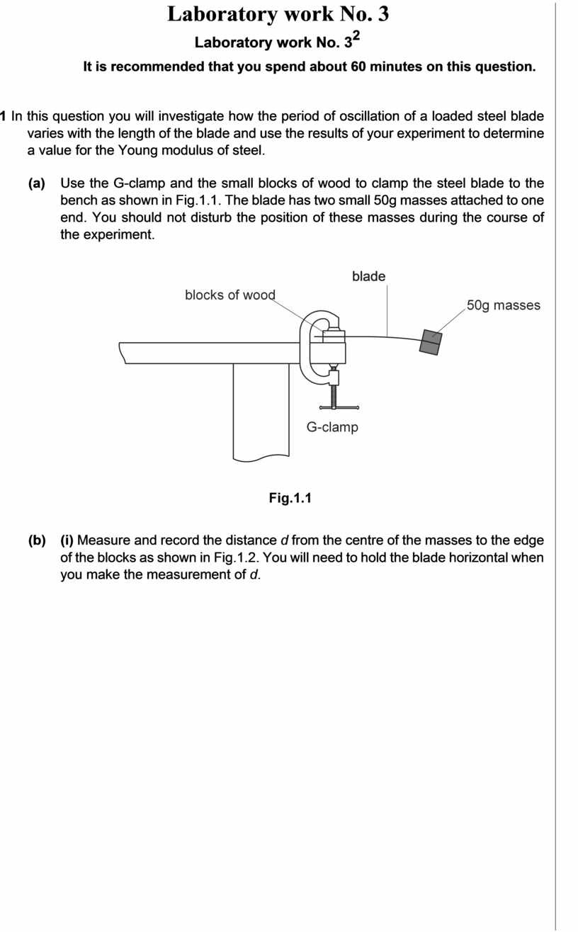
1 In this question you will investigate how the period of oscillation of a loaded steel blade varies with the length of the blade and use the results of your experiment to determine a value for the Young modulus of steel.
(a) Use the G-clamp and the small blocks of wood to clamp the steel blade to the bench as shown in Fig.1.1. The blade has two small 50g masses attached to one end. You should not disturb the position of these masses during the course of the experiment.
![]() blade
blade

(b) (i) Measure and record the distance d from the centre of the masses to the edge of the blocks as shown in Fig.1.2. You will need to hold the blade horizontal when you make the measurement of d.

![]() Fig.1.2
Fig.1.2
d = ........................................................... m
(ii) Displace the end of the blade from its equilibrium position and release it so that the strip performs small oscillations in a vertical plane. Make and record measurements to determine the period T of oscillation of the blade.
T = ............................................................ s
4
(c) Change the value of d and repeat (b)(i) and (ii) until you have six sets of readings of distance d and period T for values of d in the range 0.130m < d < 0.250m.
|
|
|
|
|
|
|
|
|
|
|
|
![]() Include in your table of results all six
sets of values for lg (T/s) and lg (d/m).
Include in your table of results all six
sets of values for lg (T/s) and lg (d/m).
(d) (i) Plot a graph of lg (T/s) (y-axis) against lg (d/m) (x-axis).
(ii) Draw the line of best fit.
(iii) Determine the gradient and the y-intercept of this line.
|
|
|
gradient
= ...................................................... y-intercept =
...................................................... 5 ![]()
6
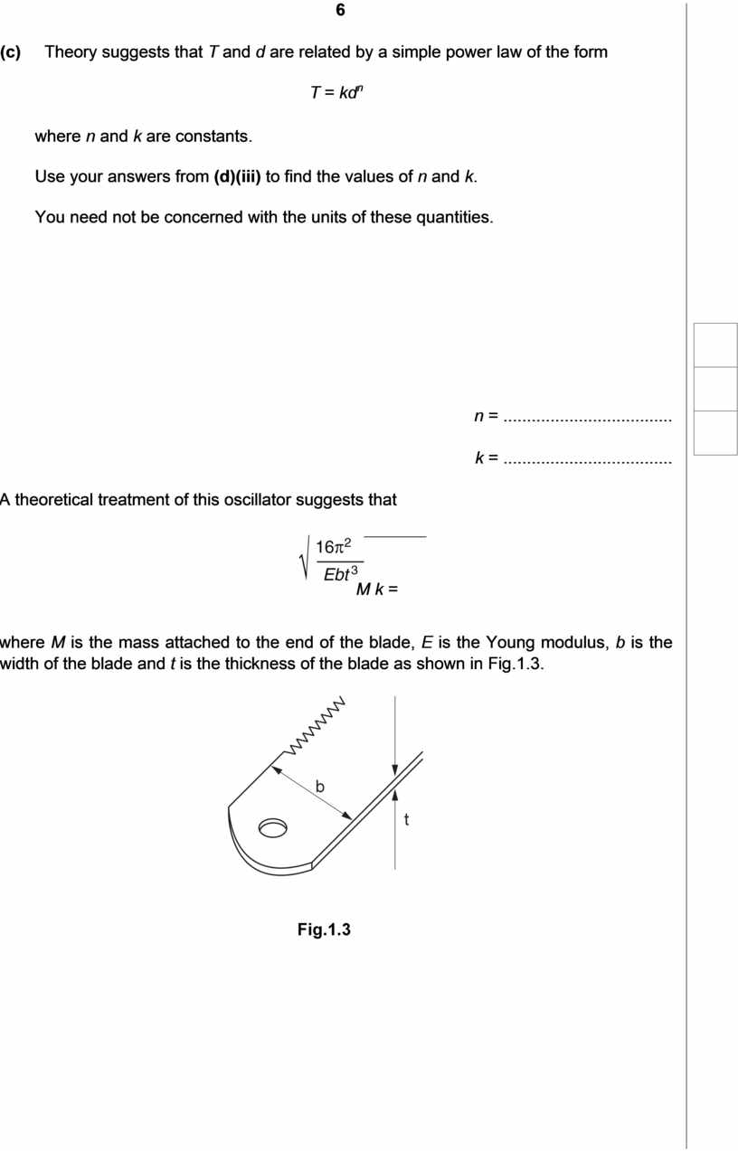
(e) Theory suggests that T and d are related by a simple power law of the form
T = kdn
where n and k are constants.
Use your answers from (d)(iii) to find the values of n and k.
|
|
|
|
|
|
![]() You need not be concerned with the units
of these quantities.
You need not be concerned with the units
of these quantities.
n = ....................................
k = ....................................
A theoretical treatment of this oscillator suggests that
![]()
![]() M k =
M k =
where M is the mass attached to the end of the blade, E is the Young modulus, b is the width of the blade and t is the thickness of the blade as shown in Fig.1.3.
![]() 7
7
(f) (i) Measure the values of b and t. The measurement of t should be made on a part of the blade where there is no tape.
b = ......................................... m t = ......................................... m
(ii) State the name of the instrument used to measure t.
..................................................................................................................................
(iii) Estimate the percentage uncertainty in the value of t 3.
percentage uncertainty in t 3 = ........................................ %
(g) Determine a value for E. Include an appropriate unit.
E = ...............................................................
![]()
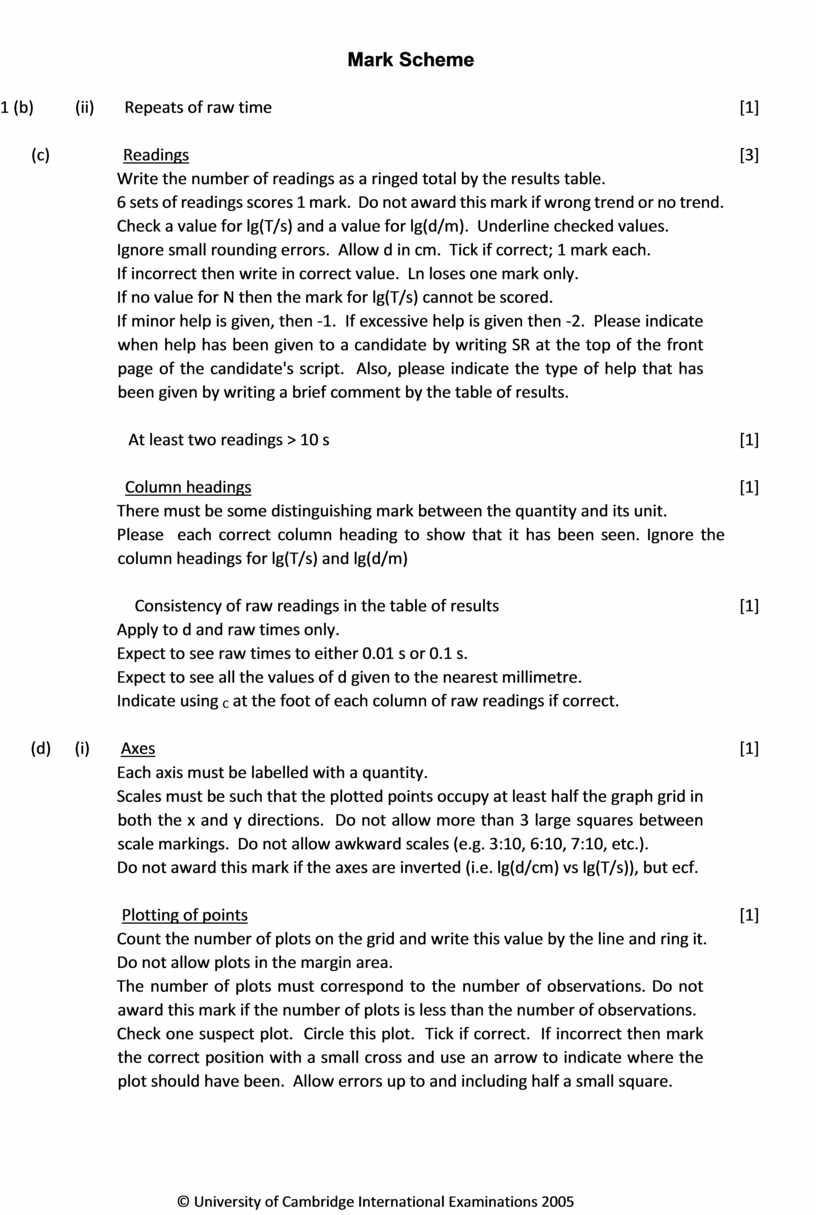
1 (b) (ii) Repeats of raw time [1]
(c) Readings [3]
Write the number of readings as a ringed total by the results table.
6 sets of readings scores 1 mark. Do not award this mark if wrong trend or no trend.
Check a value for lg(T/s) and a value for lg(d/m). Underline checked values.
Ignore small rounding errors. Allow d in cm. Tick if correct; 1 mark each.
If incorrect then write in correct value. Ln loses one mark only.
If no value for N then the mark for lg(T/s) cannot be scored.
If minor help is given, then -1. If excessive help is given then -2. Please indicate when help has been given to a candidate by writing SR at the top of the front page of the candidate's script. Also, please indicate the type of help that has been given by writing a brief comment by the table of results.
At least two readings > 10 s [1]
Column headings [1]
There must be some distinguishing mark between the quantity and its unit.
Please each correct column heading to show that it has been seen. Ignore the column headings for lg(T/s) and lg(d/m)
Consistency of raw readings in the table of results [1]
Apply to d and raw times only.
Expect to see raw times to either 0.01 s or 0.1 s.
Expect to see all the values of d given to the nearest millimetre.
Indicate using C at the foot of each column of raw readings if correct.
(d) (i) Axes [1]
Each axis must be labelled with a quantity.
Scales must be such that the plotted points occupy at least half the graph grid in both the x and y directions. Do not allow more than 3 large squares between scale markings. Do not allow awkward scales (e.g. 3:10, 6:10, 7:10, etc.).
Do not award this mark if the axes are inverted (i.e. lg(d/cm) vs lg(T/s)), but ecf.
Plotting of points [1]
Count the number of plots on the grid and write this value by the line and ring it.
Do not allow plots in the margin area.
The number of plots must correspond to the number of observations. Do not award this mark if the number of plots is less than the number of observations.
Check one suspect plot. Circle this plot. Tick if correct. If incorrect then mark the correct position with a small cross and use an arrow to indicate where the plot should have been. Allow errors up to and including half a small square.
© University of Cambridge International Examinations 2005
![]()
(ii) Line of best fit [1]
There must be a reasonable balance of points about the line of best fit. If one of the plots is a long way from the trend of the other plots then allow this plot to be ignored when the line is drawn.
(iii) Measurement of gradient [1]
The hypotenuse of the triangle must be greater than half the length of the drawn line.
Read-offs must be accurate to half a small square and ratio must be correct.
Please indicate the vertices of the triangle used by labelling with ∆.
y-intercept [1]
Check the read-off.
Accept correct substitution from a point on the line into y = mx + c.
(e) lg T = n lg d + lg k [1]
This can be implied from the working.
Value for n (from gradient) [1]
Value for k (only from 10y-intercept) [1]
(f) (i) Value of t (±0.05 mm of SV) or ± 0.05 mm of extremes if range given [1] If POTE do not award this mark.
(ii) Micrometer screw gauge/micrometer/screw gauge [1]
(iii) Percentage uncertainty in t3 [1]
∆t ratio, x100 and ‘x 3’ must be correct.
∆t can be 0.005 mm, 0.01 mm, 0.02 mm or half the range.
(g) Value of E [1]
Check the substitution, working and consistency of units.
Must be in range from 5.0 x 10¹⁰ to 5.0 x 10¹¹ Pa.
Allow M = 0.05 kg or 0.10 kg.
Bald answer for E scores zero.
Unit of E (Pa or N m-2) [1]
[Total: 20 marks]
© University of Cambridge International Examinations 2005
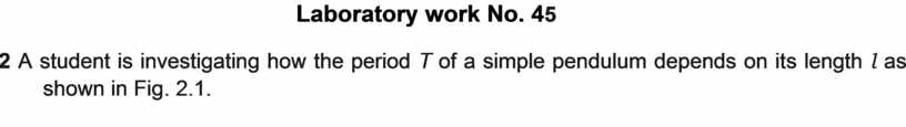
2 A student is investigating how the period T of a simple pendulum depends on its length l as shown in Fig. 2.1.
![]()
 Fig. 2.1
The time t for 10 oscillations is recorded for a pendulum of length l. The period T of the pendulum is determined. The procedure is then repeated for different lengths.
Question 2 continues on the next page.
[Turn over
6
It is suggested that T and l are related by the equation
|
l / cm |
t / s |
|
|
|
90.0 |
18.9 ± 0.1 |
|
|
|
80.0 |
17.9 ± 0.1 |
|
|
|
70.0 |
16.7 ± 0.1 |
|
|
|
60.0 |
15.5 ± 0.1 |
|
|
|
50.0 |
14.1 ± 0.1 |
|
|
|
40.0 |
12.6 ± 0.1 |
|
|
![]() T = 2π
T = 2π ![]()
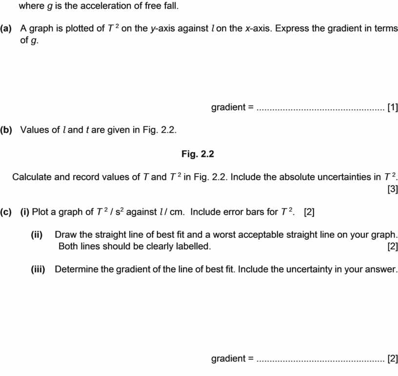
where g is the acceleration of free fall.
(a) A graph is plotted of T 2 on the y-axis against l on the x-axis. Express the gradient in terms of g.
gradient = ................................................. [1]
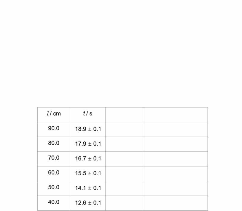
(b) Values of l and t are given in Fig. 2.2.
Fig. 2.2
Calculate and record values of T and T 2 in Fig. 2.2. Include the absolute uncertainties in T 2.
[3]
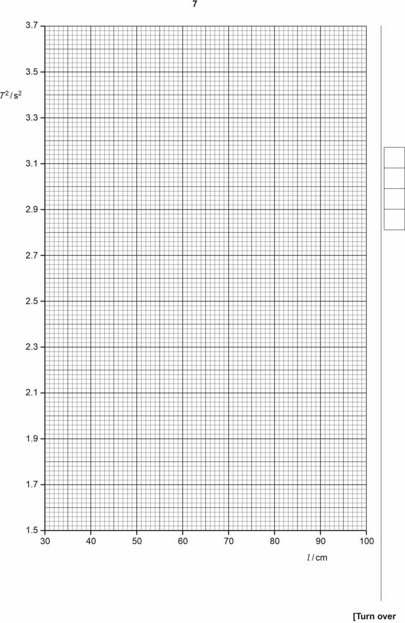
(c) (i) Plot a graph of T 2 / s2 against l / cm. Include error bars for T 2. [2]
(ii) Draw the straight line of best fit and a worst acceptable straight line on your graph.
Both lines should be clearly labelled. [2]
(iii) Determine the gradient of the line of best fit. Include the uncertainty in your answer.
gradient = ................................................. [2]
8
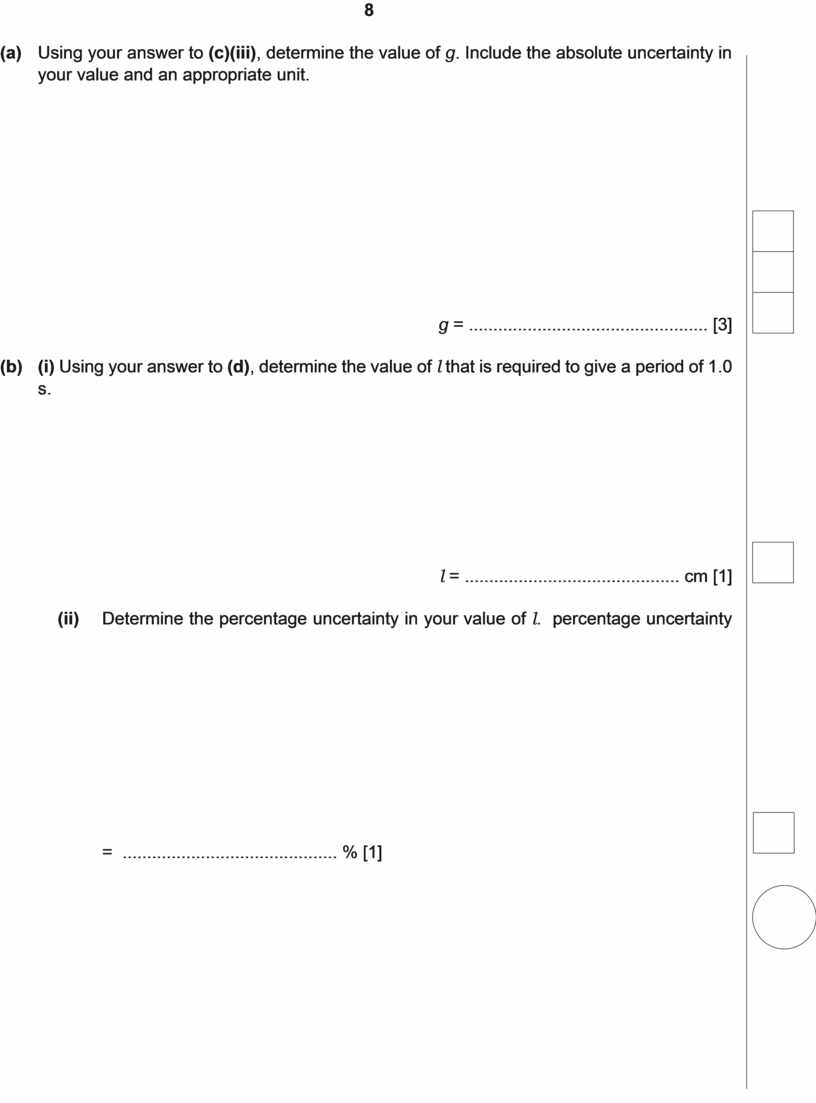
(d)  Using your answer to (c)(iii),
determine the value of g. Include the absolute uncertainty in your value
and an appropriate unit.
Using your answer to (c)(iii),
determine the value of g. Include the absolute uncertainty in your value
and an appropriate unit.
g = ................................................. [3]
(e) (i) Using your answer to (d), determine the value of l that is required to give a period of 1.0 s.
l = ............................................ cm [1]
(ii) Determine the percentage uncertainty in your value of l. percentage uncertainty = ............................................ % [1]
![]()
Permission to reproduce items where third-party owned material protected by copyright is included has been sought and cleared where possible. Every reasonable effort has been made by the publisher (UCLES) to trace copyright holders, but if any items requiring clearance have unwittingly been included, the publisher will be pleased to make amends at the earliest possible opportunity.
University of Cambridge International Examinations is part of the Cambridge Assessment Group. Cambridge Assessment is the brand name of University of Cambridge Local Examinations Syndicate (UCLES), which is itself a department of the University of Cambridge.

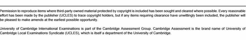
2 Analysis, conclusions and evaluation (15 marks)
|
Part |
Mark |
Expected Answer |
Additional Guidance |
||
|
(a) |
A1 |
2 4π
g |
39.5 Allow g |
||
|
(b) |
T1 |
Column headings: T / s and T 2 / s2 |
There must be a dividing mark between the quantity and the unit, i.e. “in”; “/”; (unit) e.g. T (s). |
||
|
|
T2 |
|
Must be values in the table. |
||
|
|
3.57 or 3.572 |
|
|||
|
3.20 or 3.204 |
|||||
|
2.79 or 2.789 |
|||||
|
2.40 or 2.403 |
|||||
|
1.99 or 1.988 |
|||||
|
1.59 or 1.588 |
|||||
|
|
U1 |
From ± 0.04 to ± 0.02 or ± 0.03 |
Allow more than one significant figure, e.g. ± 0.038. |
||
|
(c) (i) |
G1 |
Six points plotted correctly |
Must be within half a small square. Ecf allowed from table. |
||
|
|
U2 |
Error bars in T 2 plotted correctly. |
Check first and last point. Must be accurate within half a small square. All plots must have error bars. |
||
|
(ii) |
G2 |
Line of best fit |
If points are plotted correctly then lower end of line should pass between (37, 1.5) and (38, 1.5) and upper end of line should pass between (92, 3.7) and (94, 3.7). Allow ecf from points plotted incorrectly – examiner judgement. |
||
|
|
G3 |
Worst acceptable straight line. Steepest or shallowest possible line that passes through all the error bars. |
Line should be clearly labelled or dashed. Should pass from top of top error bar to bottom of bottom error bar or bottom of top error bar to top of bottom error bar. Mark scored only if error bars are plotted. |
||
|
(iii) |
C1 |
Gradient of best fit line |
The triangle used should be at least half the length of the drawn line. Check the read-offs. Work to half a small square. Do not penalise POT. |
||
|
|
U3 |
Error in gradient |
Method of determining absolute error. Difference in worst gradient and gradient. |
||
|
(d) |
C2 |
g = 4π2/gradient = 39.5/gradient |
Gradient must be used correctly. Allow ecf from (c)(iii). |
||
|
|
U4 |
Determines uncertainty in g |
Uses worst calculated g value or fractional method. Do not check calculation. |
||
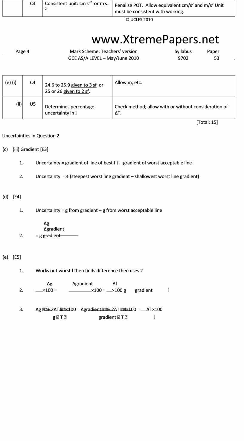
|
|
C3 |
Consistent unit: cm s–2 or m s–2 |
Penalise POT. Allow equivalent cm/s2 and m/s2 Unit must be consistent with working. |
||
© UCLES 2010
 www.XtremePapers.net
 Page 4 Mark
Scheme: Teachers’ version Syllabus Paper
Page 4 Mark
Scheme: Teachers’ version Syllabus Paper
GCE AS/A LEVEL – May/June 2010 9702 53
|
(e) (i) |
C4 |
24.6 to 25.9 given to 3 sf or 25 or 26 given to 2 sf. |
Allow m, etc. |
|
(ii) |
U5 |
Determines percentage uncertainty in l |
Check method; allow with or without consideration of ∆T. |
[Total: 15]
Uncertainties in Question 2
(c) (iii) Gradient [E3]
1. Uncertainty = gradient of line of best fit – gradient of worst acceptable line
2. Uncertainty = ½ (steepest worst line gradient – shallowest worst line gradient)
(d) [E4]
1. Uncertainty = g from gradient – g from worst acceptable line
∆g ∆gradient
2.
![]() = g gradient
= g gradient
(e) [E5]
1. Works out worst l then finds difference then uses 2
∆g ∆gradient ∆l
2.
![]() ×100 =
×100 = ![]() ×100
=
×100
= ![]() ×100 g gradient l
×100 g gradient l
3.
![]()
![]() ∆g
+ 2∆T ×100 = ∆gradient
+ 2∆T ×100 =
∆g
+ 2∆T ×100 = ∆gradient
+ 2∆T ×100 = ![]() ∆l ×100
∆l ×100
g T gradient T l
© UCLES 2010
 www.XtremePapers.net
![]()
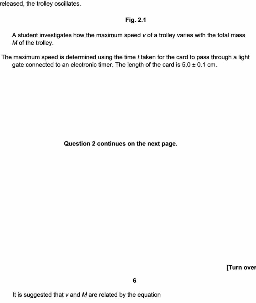
 2 A trolley is attached to springs, as shown in Fig 2.1. When
the trolley is displaced and then released, the trolley oscillates.
2 A trolley is attached to springs, as shown in Fig 2.1. When
the trolley is displaced and then released, the trolley oscillates.
Fig. 2.1
A student investigates how the maximum speed v of a trolley varies with the total mass M of the trolley.
The maximum speed is determined using the time t taken for the card to pass through a light gate connected to an electronic timer. The length of the card is 5.0 ± 0.1 cm.
Question 2 continues on the next page.
[Turn over
6
It is suggested that v and M are related by the equation
|
M / kg |
t / s |
(1/M ) / kg–1 |
v 2 / m2 s–2 |
|
0.75 |
0.046 ± 0.002 |
|
|
|
1.25 |
0.058 ± 0.002 |
|
|
|
1.75 |
0.068 ± 0.002 |
|
|
|
2.25 |
0.078 ± 0.002 |
|
|
|
2.75 |
0.086 ± 0.002 |
|
|
|
3.25 |
0.092 ± 0.002 |
|
|
![]() k
k
v = A
![]() M
M
where A is the initial displacement and k is the spring constant of the springs.
(a) A graph is plotted of v 2 on the y-axis against 1/M on the x-axis. Determine an expression for the gradient in terms of A and k.
gradient = ................................................. [1]
(b) Values of M and t are given in Fig. 2.2.
Fig. 2.2
Calculate and record values of (1/M ) / kg–1 and v 2 / m2 s–2 in Fig. 2.2. Include the absolute uncertainties in v 2. [3]
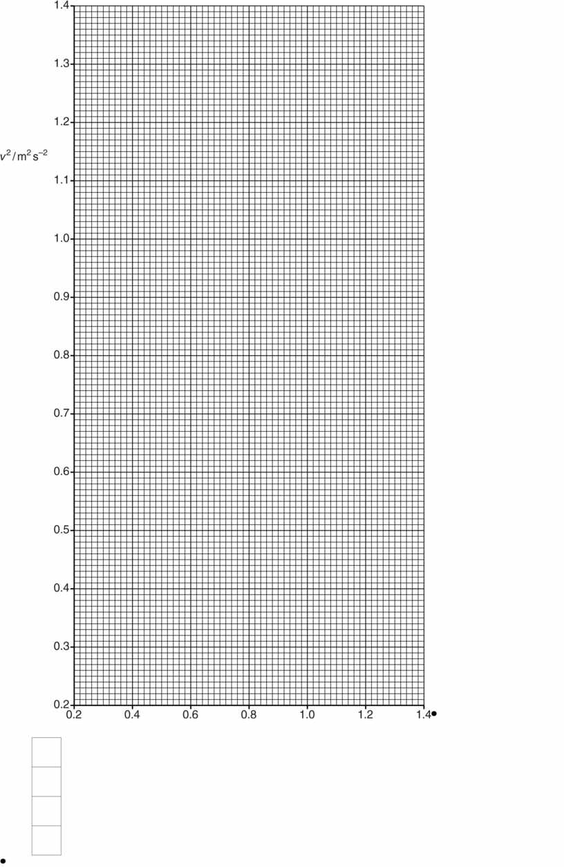
(c) (i) Plot a graph of v 2 / m2 s–2 against (1/M ) / kg–1. Include error bars for v 2. [2]
(ii) Draw the straight line of best fit and a worst acceptable straight line on your graph.
Both lines should be clearly labelled. [2]
(iii) Determine the gradient of the line of best fit. Include the uncertainty in your answer.
gradient = ................................................ [2] 7
|
|
|
(1 / M ) / kg–1 ![]()
[Turn over
8
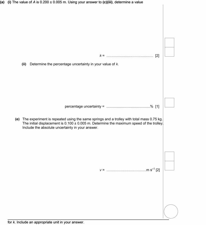
(d) (i) The value of A is 0.200 ± 0.005 m. Using your answer
to (c)(iii), determine a value  for
k. Include an appropriate unit in your answer.
for
k. Include an appropriate unit in your answer.
Permission to reproduce items where third-party owned material protected by copyright is included has been sought and cleared where possible. Every reasonable effort has been made by the publisher (UCLES) to trace copyright holders, but if any items requiring clearance have unwittingly been included, the publisher will be pleased to make amends at the earliest possible opportunity.
University of Cambridge International Examinations is part of the Cambridge Assessment Group. Cambridge Assessment is the brand name of University of Cambridge Local Examinations Syndicate (UCLES), which is itself a department of the University of Cambridge.
 Page 3 Mark
Scheme Syllabus Paper
Page 3 Mark
Scheme Syllabus Paper
GCE AS/A LEVEL – October/November 2012 9702 53
2 Analysis, conclusions and evaluation (15 marks)
|
Part |
Mark |
Expected Answer |
Additional Guidance |
||
|
(a) |
A1 |
Gradient = kA2 |
|
||
|
(b) |
T1 T2 |
|
T1 must be values in 1/M. Ignore row 2.
T2 must be to 2 s.f. or 3 s.f.
|
||
|
1.3 or 1.33 |
1.2 |
|
|||
|
0.8(0)(0)(0) |
0.74 |
||||
|
0.571 or 0.5714 |
0.54 or 0.55 |
||||
|
0.444 or 0.4444 |
0.41 or 0.411 or 0.410 |
||||
|
0.364 or 0.3636 |
0.34 |
||||
|
0.308 or 0.3077 |
0.29 or 0.30 |
||||
|
|
U1 |
From ± 0.2 or ± 0.15 to ± 0.02 or ± 0.03 |
Allow more than one significant figure. Do not allow ± 0.1 for row 1. |
||
|
(c) (i) |
G1 |
Six points plotted correctly |
Must be within half a small square. Penalise ‘blobs’. Ecf allowed from table. |
||
|
|
U2 |
All error bars in v2 plotted correctly |
Must be accurate within half a small square. |
||
|
(c) (ii) |
G2 |
Line of best fit |
There must be a balance of points about the line of best fit – examiner judgement. Allow ecf from points plotted incorrectly. |
||
|
|
G3 |
Worst acceptable straight line. Steepest or shallowest possible line that passes through all the error bars. |
Line should be clearly labelled or dashed. Should pass from top of top error bar to bottom of bottom error bar or bottom of top error bar to top of bottom error bar. Mark scored only if error bars are plotted. |
||
|
(c) (iii) |
C1 |
Gradient of best fit line
|
The triangle used should be at least half the length of the drawn line. Check the read offs. Work to half a small square. Do not penalise POT. Should be about 0.9. |
||
|
|
U3 |
Uncertainty in gradient |
Method of determining absolute uncertainty. Difference in worst gradient and gradient. |
||
|
(d) (i) |
C2 |
k = gradient / A2 = gradient / 0.04 |
Should be about 22. |
||
|
|
C3 |
N m–1 |
Allow kg s–2 |
||
|
(d) (ii) |
U4 |
Percentage uncertainty in k |
∆m ∆A ∆m
m A m |
||
© Cambridge International Examinations 2012
 Page 4 Mark
Scheme Syllabus Paper
Page 4 Mark
Scheme Syllabus Paper
GCE AS/A LEVEL – October/November 2012 9702 53
|
(e) |
C4 |
v in the range 0.534 to 0.559 and given to 2 or 3 s.f. |
For 2 s.f. 0.53 to 0.56 |
|
|
U5 |
Uncertainty in v |
|
[Total: 15]
Uncertainties in Question 2
(c) (iii) Gradient [U3]
Uncertainty = gradient of line of best fit – gradient of worst acceptable line
Uncertainty = ½ (steepest worst line gradient – shallowest worst line gradient)
(d) (ii) [U4]
|
Percentage uncertainty = max m Maximum
k = (min A) min m Minimum
k = (max A) |
∆m ∆A ∆m
|
|
|
m |
A m |
|
|
|
∆k |
(max k−min )k |
Percentage
uncertainty = ![]() ×100 =
×100 =![]()
![]() ×100 kk
×100 kk
(e) [U5]
∆A ∆k
Percentage
uncertainty = ×100+ 21× ![]() ×100
×100
A k
Absolute uncertainty = v × percentage uncertainty/100
max k
Maximum v = max A×
 0.75 min k
Minimum v = min A×
0.75
Absolute uncertainty = max v – v or v –
min v or![]() (maxv− minv)
(maxv− minv)
© Cambridge International Examinations 2012

 You may not need to use
all of the materials provided.
You may not need to use
all of the materials provided.
1 In this experiment you will measure the period of oscillation of a wooden rod weighted at different positions. You will use the results to determine the mass of the rod.
(a) Set up the rod so that it is pivoted by a nail as shown in Fig. 1.1. Another nail should be placed through the bottom hole and a 0.100 kg mass is to be held in place with a small piece of Blu-Tack.
(b) Measure the distance l between the two nails.
l = .................................................. m
(c) Displace the rod so that it oscillates with a small amplitude in a vertical plane as shown in Fig. 1.2.
Determine the period T of oscillation.
T = ................................................... s
[Turn over
4
(d) ![]() Move the bottom nail and
the mass to different holes and repeat (b) and (c) until you have
six sets of readings for l and T. Include values for T 2 in your
table of results.
Move the bottom nail and
the mass to different holes and repeat (b) and (c) until you have
six sets of readings for l and T. Include values for T 2 in your
table of results.
(e) Plot a graph of T 2 on the y-axis against l on the x-axis and draw the line of best fit.
(f) Determine the gradient and y-intercept of this line.
gradient = .......................................................
y-intercept = ....................................................... 5
|
|
|
|
[Turn over
6
(g) It is suggested that the relationship between T 2 and l is
4π2ml
T 2
= ![]() + z
+ z
g (m + M )
where m is 0.100 kg, M is the mass of the rod, g = 9.81 N kg –1 and z is a constant for this experiment.
![]() Use your answers from (f)
to determine the values of M and z. Give appropriate units.
Use your answers from (f)
to determine the values of M and z. Give appropriate units.
M = ....................................................... z = .......................................................

1 Manipulation, measurement and observation
Successful collection of data
|
(b) Value of length 0.470m to 0.490m (to nearest cm or mm).
|
[1] |
|
(c) 10T (or more) has been measured (could be evidence in table of results).
|
[1] |
|
(c) Repeat readings. At least two readings of 10T or T (could be in table).
(d) Results Write the number of readings as a ringed total next to the table of results. Six sets of values for T and l scores 3 marks, five sets scores 2 marks. |
[1] |
|
If raw data shows reverse trend then –1.
|
[3] |
|
(d) Apparatus set up without help from Supervisor.
Range and distribution of values
(d) Range of results (including the value in (b)). |
[1] |
|
Must include 48cm and 18cm (nominal values), with no interval greater than 7cm.
Presentation of data and observations
Table: layout
(d) Column headings. Each column heading must contain a quantity and a unit where appropriate. Ignore units in the body of the table. There must be some distinguishing mark between the quantity and the unit |
[1] |
|
(solidus is expected, but accept, for example, T (s)).
Table: raw data
(d) Consistency of presentation of raw readings. All values of 10T (or T) must be given to the same number of decimal places. |
[1] |
|
If these are to the nearest second then –1. Allow trailing zeros.
Table: calculated quantities
(d) Significant figures. Apply toT ². Take trailing zeros into account. If 10T is given to 2 sf, then accept T ² to 2 or 3 sf. If 10T is given to 3 sf, then accept T ² to 3 or 4 sf. |
[1] |
|
If 10T is given to 4 sf, then accept T ² to 4 or 5 sf.
(d) Values of T ² correct. |
[1] |
|
Check a value (from candidate’s T). If incorrect, write in the correct value. |
[1] |
© UCLES 2008

Graph: layout
(Graph) Axes.
Sensible scales must be used (not 3:10 etc.), with labels at least every three large squares.
Scales must be such that the plotted points occupy at least half the graph grid in both x and y directions.
Scales must be labelled with the quantity which is being plotted. Ignore units.
Indicate false origin with FO.
Allow reversed axes, but if wrong graph plotted then –1. [1]
Graph: plotting of points
(Graph) All observations must be plotted. Count and circle the number of plots.
Ring and check a suspect plot. Tick if correct. Re-plot if incorrect.
Work to an accuracy of half a small square.
Don’t allow blobs (i.e. large dots with diameter ≥ half a small square). [1]
Graph: trend line
(Graph) Line of best fit. Allow 5 trend plots.
Judge by scatter of points about the candidate's line.
Indicate best line if candidate's line is not the best line.
Don’t allow a line thicker than half a small square. [1]
Quality of data
(Graph) Judge by scatter of points.
Allow 2cm (scaled) in the l direction either side of any line that could be drawn.
All plots from table are needed for this mark to be scored.
Do not award this mark if the trend is wrong or if wrong graph is drawn. [1]
Analysis, conclusions and evaluation
Interpretation of graph
(f) Gradient.
The hypotenuse of the ∆ must be ≥ half the length of the drawn line.
Read-offs must be accurate to half a small square.
Check for ∆y/∆x (do not allow ∆x/∆y). [1]
(f) The y-intercept value must be read to the nearest half square.
Check for false origin. The value can be calculated using ratios or y = mx + c. [1]
Drawing conclusions
(g) Value for M. Check substitution into “gradient = 4π2m/g(m+M)” is correct.
Allow 10 – 70g. Unit required. [1]
(g) Value for z. Must equal the y-intercept. Unit required (s2). 2 or 3 s.f. [1]
[Total: 20]
© UCLES 2008
NIS Taldykorgan Names ____________________________________
Grade 11 Physics Class/Section _______________________________
Gas Law simulation; Investigating Boyle’s Law
Task: You are to use the Phet simulation to collect data and make a graph that relates the pressure of a gas to the volume the gas occupies.
Background: Learn how to adjust the macroscopic properties in the gas simulation by watching the 4 minute simulation at http://www.youtube.com/watch?v=EzWRvK0zhQk .
Activity: Set your temperature and number of molecules at fixed amount and keep them constant. To adjust the volume, move the man and record the length of your container. Calculate the volume of the container in meter3 by assuming the container is a square with the same dimensions. Record the pressure for each of 10 data points. Fill in the data table including the missing units. Use your data to complete a graph. Be sure to add a tile, scales, labels and units!
Data: Using the Phet simulation at http://phet.colorado.edu/en/simulation/gas-properties collect a set of data, fill in the data table.
|
|
|
Data Analysis: Answer the following questions:
What was your independent variable? _________________________________________________________
What was your dependent Variable? ___________________________________________________________
What did you have to keep constant (your controlled variables)? _____________________________________
On the graph, what axis does the independent variable go on? _______________________________________
What is the shape of your graph? ______________________________________________________________
What do we call this kind of relationship? ________________________________________________________
Reflection:
For a real gas, the shape of the Volume vs. Pressure graph is a slightly curved line. Think about the difference between your simulation, a real gas and an ideal gas. Propose an explanation using scientific terminology. __________________________________________________________________________________________ __________________________________________________________________________________________
__________________________________________________________________________________________ __________________________________________________________________________________________
__________________________________________________________________________________________
36
NIS Taldykorgan Names ____________________________________
Grade 11 Physics Class/Section _______________________________
Gas Law simulation; Investigating Gay-Lussac’s Law
Task: You are to use the Phet simulation to collect data and make a graph that relates the pressure of a gas to the temperature the gas occupies.
Background: Learn how to adjust the macroscopic properties in the gas simulation by watching the 4 minute simulation at http://www.youtube.com/watch?v=EzWRvK0zhQk
Data: Using the Phet simulation at http://phet.colorado.edu/en/simulation/gas-properties collect a set of data, fill in the data table.
|
|
|
Data Analysis: Answer the following questions:
What was your independent variable? _________________________________________________________
What was your dependent Variable? ___________________________________________________________
What did you have to keep constant (your controlled variables)? _____________________________________
On the graph, what axis does the independent variable go on? _______________________________________
What is the shape of your graph? ______________________________________________________________
What do we call this kind of relationship? ________________________________________________________
37
![]() card
card
![]()
![]()
![]() Suspend one paper clip from the loop, as
shown in Fig. 2.2.
Suspend one paper clip from the loop, as
shown in Fig. 2.2.
Fig. 2.2 (NOT TO SCALE)
(a) (i) Measure and record the angle (as shown in Fig. 2.2) between your plumb line and the 90° line on your protractor image.
= [1]
(ii) Repeat (a)(i) using different numbers n of paper clips.
Record all of your results in a table in the space below.
[2]
(iii) Using the grid in Fig. 2.3, plot a graph of on the y-axis against n on the x-axis.
![]()
|
|
[2] |
|
(iv) Draw the smooth curve of best fit through the plotted points. |
[1] |
(b) Remove the paper clips so that the loop is horizontal as in Fig. 2.1.
• Slowly raise the beaker of water until all of the loop is in contact with the water surface.
• Slowly move the beaker vertically downwards. At first the loop moves down with the water surface.
(i) Record the value of just as the loop separates from the water surface.
= [2]
![]()
(ii) ![]()
![]()
![]() Use your graph to find the value of n
corresponding to the value found in (b)(i).
Use your graph to find the value of n
corresponding to the value found in (b)(i).
n = [1]
(iii) Calculate the force F needed to separate the loop from the water surface by using the expression
F = n m g
where:
n is the value from (b)(ii) m is the mass (in kg) of one paper clip (written on a card taped to the stand) g = 9.81 m s–2.
F = N [1]
(c) Unhook the wire loop from the card.
(i) Take measurements to find the diameter D of the loop, as shown in Fig. 2.4.

Side view Top view
Fig. 2.4 (NOT TO SCALE)
![]()
D = cm [2]
![]()
(ii) Calculate the surface tension of the water by using the expression
F
= ![]()
2D
Give your answer to a suitable number of significant figures.
= N cm–1 [2]
![]()
Mark Scheme
|
Question |
Answer |
AO |
Mark |
Additional Guidance |
|
2(a)(i) |
in range 2 to 20 |
AO3 |
B1
[1] |
|
|
2(a)(ii) |
table drawn with columns and headings for n and
at least four sets of n and |
AO3
AO3 |
B1
B1
[2] |
ignore missing or incorrect units |
|
2(a)(iii) |
axes labelled correctly
points plotted correctly |
AO2
AO3 |
B1
B1
[2] |
|
|
2(a)(iv) |
smooth curve plotted through points |
AO2 |
B1
[1] |
|
|
2(b)(i) |
value for in range 5 to 20
evidence of repeated measurements of |
AO3
AO3 |
B1
B1
[2] |
|
|
2(b)(ii) |
correct reading of n from graph |
AO2 |
B1
[1] |
accept to nearest integer value ecf from (b)(i) |
|
2(b)(iii) |
correct calculation of F |
AO3 |
B1
[1] |
ecf from (b)(i) |
|
2(c)(i) |
readings of D to nearest mm
evidence of repeated measurements of D |
AO3
AO3 |
B1
B1
[2] |
accept to nearest 0.1 mm for a mean value |
|
2(c)(ii) |
correct calculation of
suitable number of sig. figs. for |
AO3
AO3 |
B1
B1
[2] |
accept 1 or 2 sig. figs. if n has 1 sig. fig., 2 or 3 sig. figs. if n has 2 sig. figs. ecf from (b)(iii) |
|
2(d)(i) |
any three sources of error from:
loop not circular
plumb line swings continuously
loop tends to move to side of beaker
difficult to judge at the moment the loop breaks away
parallax error between the plumb line and protractor scale
not all paper clips are identical
paper clips are too heavy so the change in is too large
value of with water is small
ripples on water surface |
AO3 |
B3
[max 3] |
|
|
2(d)(ii) |
any three improvements from:
form loop around circular pipe
damp motion of plumb line
use larger diameter beaker
record video with protractor image in view
minimise distance between plumb line and protractor scale / use lamp to form shadow of plumb line on scale
check the mass of each paper clip
use lighter / smaller paper clips to get more readings
use a bigger loop (for a bigger value of with water) / lower density or thinner card / cut to have less height
use shorter plumb line
use a platform stand for beaker |
AO3 |
B3
[max 3] |
|
Sources of information:
1. https://papers.xtremepape.rs/CAIE/AS%20and%20A%20Level/Physics%20 (9702)/
2. https://phet.colorado.edu/en/simulations/filter?subjects=physics&sort=alpha
&view=grid
3. http://files.school-collection.edu.ru/dlrstore/8e0ae370-086e-67eb-ffd452a64f02e0ce/00144678398871459.htm
4. Edexcel AS and A level/ Physics1/ Miles Hudson/2015
5. Edexcel A2 Physics /Miles Hudson/2015
6. Physics Revision Guide / Richard Woodside/2011
7. Calculations for A-level Physics /T.L.Lowe, J.F.Rounce/2002


![Line of best fit [1]](https://fs.znanio.ru/d5af0e/7c/16/c33083aab5fadab18bb5459c44fc82c22b.jpg)


Материалы на данной страницы взяты из открытых источников либо размещены пользователем в соответствии с договором-офертой сайта. Вы можете сообщить о нарушении.