ict

MOU SOSH №4 in Navoloki

Informatics lesson

"Solving equations in MS Excel"

(basic level - grade 10)

Lesson author:

 Rozanova E.F., teacher of informatics

I qual. categories.

The purpose of the lesson: Learn to use spreadsheets to graphically solve trigonometric equations.

Theoretical part

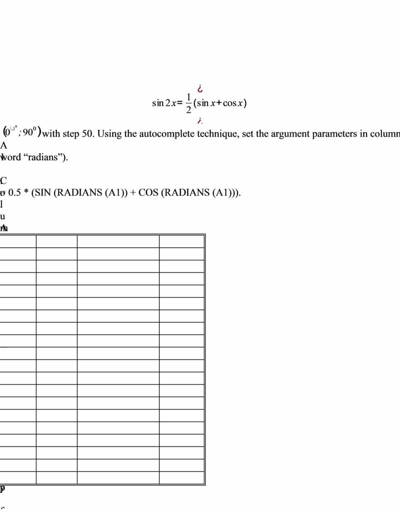
Building a graph of any function in MS Excel begins with a table setting of this function. This moment is key and predetermines the successful completion of the problem being solved. To define a function in a table, it is necessary to select the range and step of changing the argument, build the corresponding table (you can use the Edit - Fill - Progression menu, set the type of progression, step and maximum value).

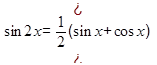
Example 1. Solve the equation (00 <X <900) graphically:

Decision. Let the argument x vary in the range with step 50. Using the autocomplete technique, set the argument parameters in column A1 ... Ap. In column В1 ... Вр enter the formula for calculating the values ​​of the function... It should be noted that in MS Excel the arguments of trigonometric functions are specified not in degrees, but in radians. Therefore, the formula in cell B1 will look like this:

= sin (radians (2 * A1)) (manually enter the word “radians”).

After typing the formula, copy it down to the end of the argument values.

Column C1 ... Wed similarly fill in the values ​​of the function , i.e.

= 0.5 * (SIN (RADIANS (A1)) + COS (RADIANS (A1))).

The calculation table will take the form:

After filling in the table, you can build graphs of functions. For this you need:

1.      Select a range of cells (B1-B19) and in the menu Insert - Chart - Custom - Smooth charts - Next;

2.      In the "Chart Data Sources" dialog box, go to the "Series" tab and press the "Add" button. Move the cursor to the "Values" field and select cells C1-C19 of the table (the inscription Sheet1! $ C $ 1: $ C $ 19 will appear). Similarly, fill in the field "Signatures by x" (position the cursor in the field and select cells A1-A19) and click the "Next" button.

3.      You can fill out the legend (you can skip it) and click the Next button, then Finish.

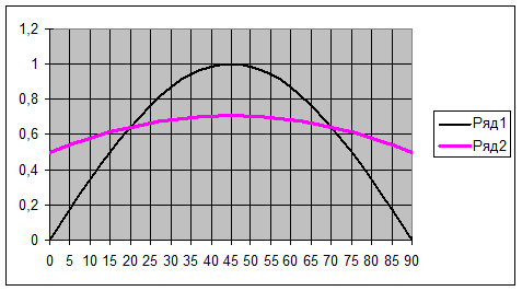
Answer x = 200,700

If the resulting schedule does not meet your requirements, then you need to return to the original table and make the necessary changes.

Practical part (for independent implementation)

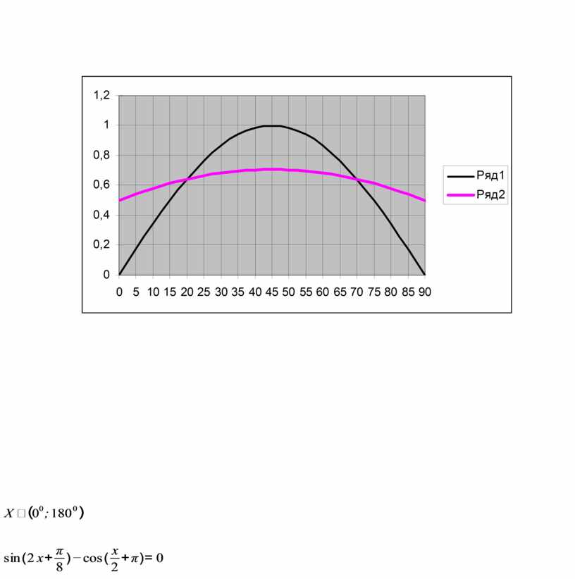
Exercise 1. Solve the equation (00 <X <900) graphically:

Assignment 2... Solve the equation graphically by changing the argument range from 00 to 1800, leaving the step the same.

Task 3. Solve the equation graphically if the argument range is from 00 to 1800 and the step is 100.

Assignment 4... Compare the results of tasks 1-3 and explain the results.

Assignment 5... Solve the equation graphically if