APPLIED PROGRAMMING IN EXCEL

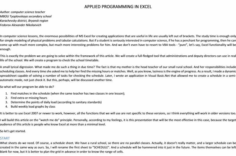
Author: computer science teacher

MBOU Tyoplovskaya secondary school

Karachevsky district, Bryansk region

Fedorov Alexander Nikolaevich

In computer science lessons, the enormous possibilities of MS Excel for creating applications that are useful in life are usually left out of brackets. The study time is enough only for simple modeling of physical problems and tabular calculations. But if a student is seriously interested in computer science, if he has a penchant for programming, then he can come up with much more complex, but much more interesting problems for him. And we don't even have to resort to VBA tools - “pure”, let's say, Excel functionality will be enough.

This is exactly the problem we are going to solve within the framework of this article. We will create a full-fledged tool that administrations and deputy directors can use in real life of the school. We will create a program to check the school timetable.

A small lyrical digression. What made me do such a thing in due time? The fact is that my mother is the head teacher of our small rural school. And her responsibilities include scheduling classes. And every time she asked me to help her find the missing hours or matches. Well, as you know, laziness is the engine of progress. As a result, I made a dynamic spreadsheet capable of solving a number of tasks for checking the schedule. Later, I wrote an application in Visual Basic.Net that allowed me to create a schedule in a semi-automatic mode, not just check it. But this, perhaps, will be discussed another time.

So what will our program be able to do?

1.       Find matches in the schedule (when the same teacher has two classes in one lesson);

2.       Find extra or missing hours

3.       Determine the points of daily load (according to sanitary standards)

4.       Build weekly load graphs by class

It is better to use Excel 2007 or newer to work, however, all the functions that we will use are not specific to these versions, so I think everything will work in older versions too.

I will build this article on the "watch me do" principle. Personally, according to my feelings, it is this presentation that will be the most effective in this case, because the target audience of this article is people who know Excel at more than a minimal level.

So let's get started.

START

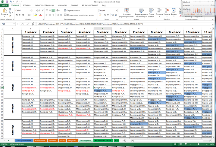
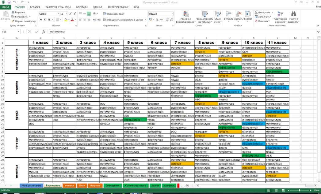
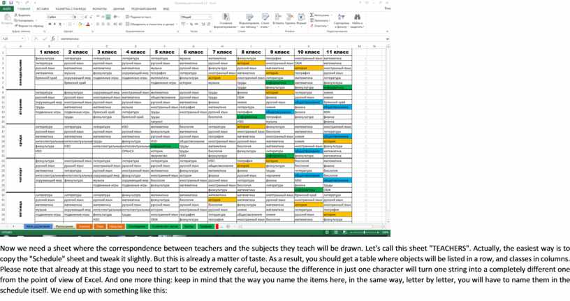
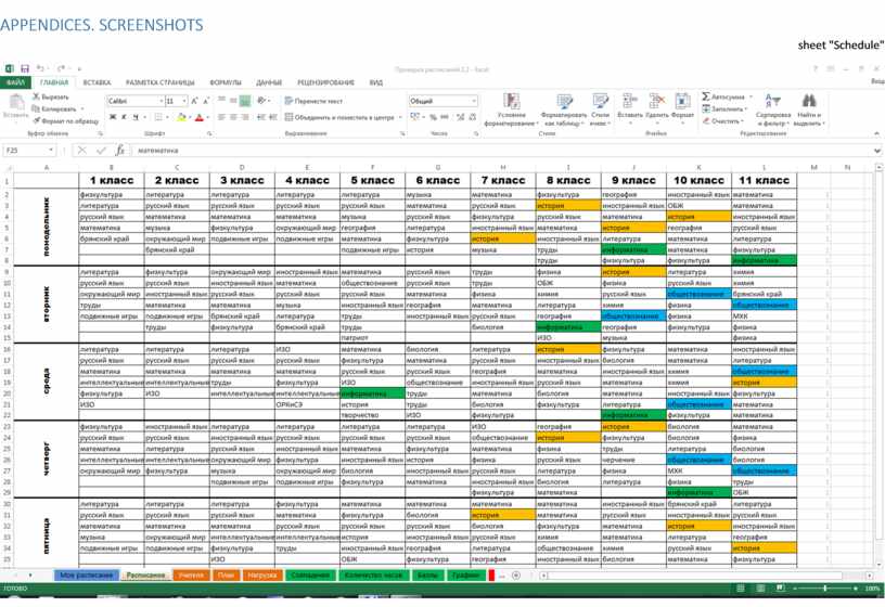
What sheets do we need. Of course, a schedule sheet. We have a rural school, so there are no parallel classes. Actually, it doesn't really matter, and a larger schedule can be created in the same way as ours. So, I will rename the first sheet to "SCHEDULE". And a schedule will be hammered into it just in the future. The items themselves can be left blank for now, but it is better to plan the grid in advance in order to know the range of cells.

The blue, yellow and green cells in the screenshot are my lessons. I did it for myself, I don’t need to pay attention to it yet. Normal conditional cell formatting, and we'll talk about that later.

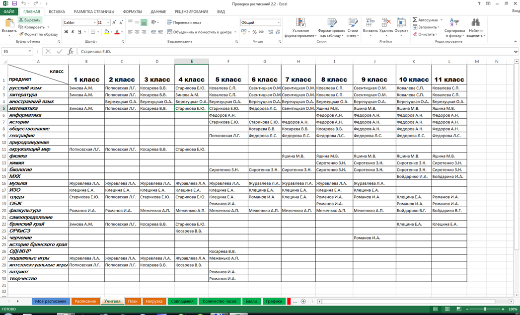
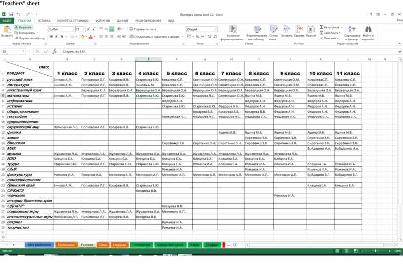
Now we need a sheet where the correspondence between teachers and the subjects they teach will be drawn. Let's call this sheet "TEACHERS". Actually, the easiest way is to copy the "Schedule" sheet and tweak it slightly. But this is already a matter of taste. As a result, you should get a table where objects will be listed in a row, and classes in columns. Please note that already at this stage you need to start to be extremely careful, because the difference in just one character will turn one string into a completely different one from the point of view of Excel. And one more thing: keep in mind that the way you name the items here, in the same way, letter by letter, you will have to name them in the schedule itself. We end up with something like this:

WE CARRY OUT COINCIDENCE CHECK

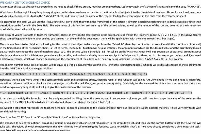
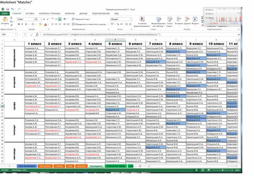
As a matter of fact, we already have everything we need to check if there are any matches among teachers. Let's copy again the "Schedule" sheet and name this copy "MATCHES".

What is our further logic? Everything is very simple - on this sheet we have to transform the timetable of subjects into the timetable of teachers. Those. for each cell, we check which subject corresponds to it in the "Schedule" sheet, and then we find the name of the teacher leading the given subject in this class from the "Teachers" sheet.

To accomplish this task, we will use the INDEX function. I don’t think that within the framework of this article it is worth describing each function in detail, especially since their description can be found in the Excel Help. The arguments of this function are: an array of the desired values, as well as the number of the row and column, at the intersection of which the same value will be found.

The array of values ​​is a table of teachers' surnames. Those. in my specific case (shown in the screenshots) it will be the Teacher's range! $ B $ 2: $ L $ 30 (if the above figures show something poorly due to poor quality, you can see it at the end of the document - there will be applications with the same screenshots, but larger).

The row number is to be obtained by looking for the name of the subject (which we get from the "Schedule" sheet by coordinates that coincide with the coordinate of our cell) in the first column of the "Teachers" sheet, i.e. list of items. The SEARCH function will help us with this, the arguments of which are the desired value and the array being looked up. Naturally, we choose the type of matching equal to 0. The desired value is Schedule! B2 (for cell B2 on the Matches sheet). I will not arrange an educational program about absolute and relative links, I think everyone already knows this, and understands why in some cases I put the $ sign, and in others not. In this case, as you understand, I just need a relative reference, which will change depending on the coordinates of the edited cell. The array being looked up is Teachers! $ A $ 2: $ A $ 30, i.e. first column.

The column number in our case, of course, will be equal to 1 (for 1 class; 2 for the second, etc., I think this is understandable). What do we get by substituting all these arguments into the INDEX function? And we get this line:

= INDEX (Teachers! $ B $ 2: $ L $ 30; SEARCH (Schedule! B2; Teachers! $ A $ 2: $ A $ 30; 0); 1)

However, there is one more thing: if the corresponding cell in the schedule is empty, then the result of this function will be # N / A! Do we need it? We don't need it. Therefore, we will introduce an additional check - is there any object at all in this cell. If not, just print an empty string. Obviously, for this we need the IF function. I am sure that there is no need to explain anything at all, so I will just give the final version of the formula.

= IF (Schedule! B2 <> ""; INDEX (Teachers! $ B $ 2: $ L $ 30; SEARCH (Schedule! B2; Teachers! $ A $ 2: $ A $ 30; 0); 1); "")

It remains to multiply this formula. It can be easily extended by filling the entire column, and in subsequent columns you will have to change the value of the column - the argument of the INDEX function (which we talked about above), i.e. change the value 1 to 2, 3, 4 ...

So, we got a table that represents the teachers' schedule, compiled according to the lesson schedule. Now our task is to visualize possible matches. This is very easy to do with conditional formatting.

Select the line B2: L2. Select the "Create Rule" item in the Conditional Formatting button.

We will need to select the option "Format only unique or duplicate values", select "Duplicate" in the drop-down list, and then use the Format button to set the view that will take cells, the values ​​of which coincide within this row. I limited myself to making the font red. Quite noticeable. That's all - we have already completed a very important task - now Excel will very clearly show us where we made a mistake.

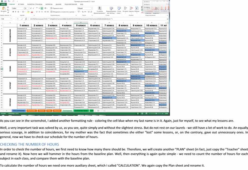
As you can see in the screenshot, I added another formatting rule - coloring the cell blue when my last name is in it. Again, just for myself, to see what my lessons are.

Well, a very important task was solved by us, as you see, quite simply and without the slightest stress. But do not rest on our laurels - we still have a lot of work to do. An equally serious scourge, in addition to coincidences, for my mother was the fact that sometimes she either "lost" some lessons, or, on the contrary, gave out unnecessary ones. In general, now we have to check our schedule for the number of hours.

CHECKING THE NUMBER OF HOURS

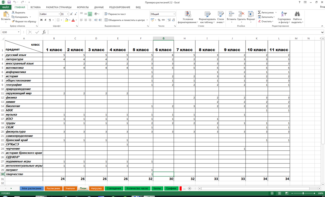
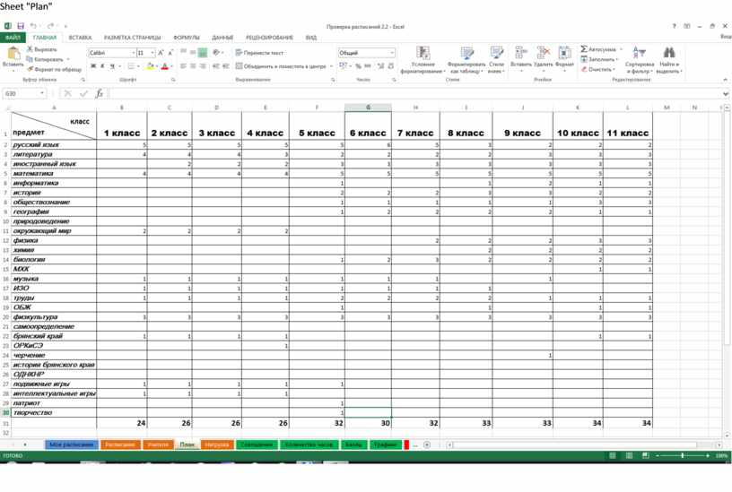
In order to check the number of hours, we first need to know how many there should be. Therefore, we will create another "PLAN" sheet (in fact, just copy the "Teacher" sheet and rename it). Now here we will hammer in the hours from the baseline plan. Well, then everything is again quite simple - we need to count the number of hours for each subject in each class, and compare them with the baseline plan.

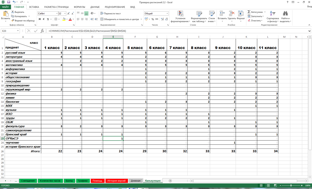
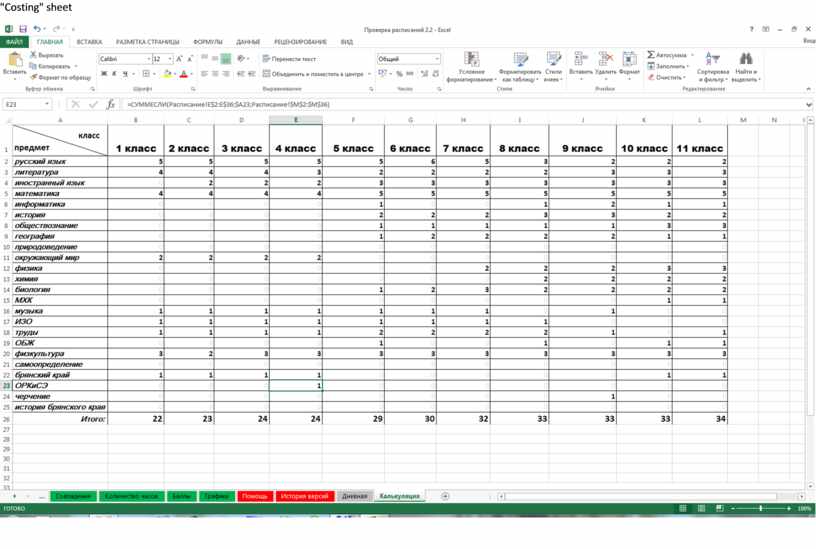
To calculate the number of hours we need one more auxiliary sheet, which I called "CALCULATION". We again copy the Plan sheet and rename it.

So, we have to count the number of hours for a subject in the class. To do this, we will use the SUMIF function. The arguments to this function are: search range, search criterion, and summation range.

The search range for cell B2 is Schedule! B $ 2: B $ 36. By the coordinates of the column, the links were left relative to make it easier to multiply. Those. we take an array of class 1 items.

The search criterion, of course, will be the name of the subject. In our case, the value of cell $ A2.

Now about the range of summation. Here we have to go for a little trick. On the "Schedule" sheet, in the M column, put 1s opposite each line of the schedule, i.e. in our example, this would be the range $ M $ 2: $ M $ 36. The font color of these units can be made white so that they are not visible. Actually, now this will be our summation range - Schedule! $ M $ 2: $ M $ 36.

Let's plug everything into the formula:

= SUMIF (Schedule! B $ 2: B $ 36; $ A2; Schedule! $ M $ 2: $ M $ 36)

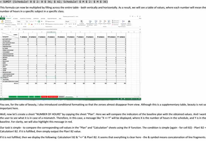
This formula can now be multiplied by filling across the entire table - both vertically and horizontally. As a result, we will see a table of values, where each number will mean the number of hours in a specific subject in a specific class.

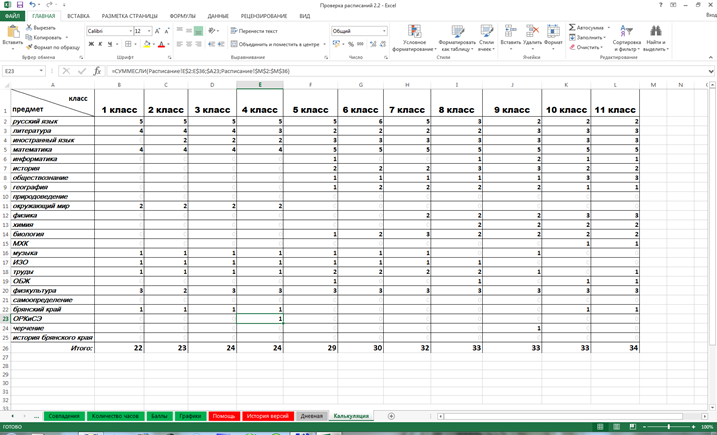
You see, for the sake of beauty, I also introduced conditional formatting so that the zeroes almost disappear from view. Although this is a supplementary table, beauty is not so important here.

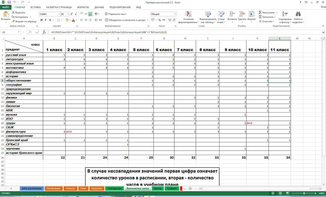
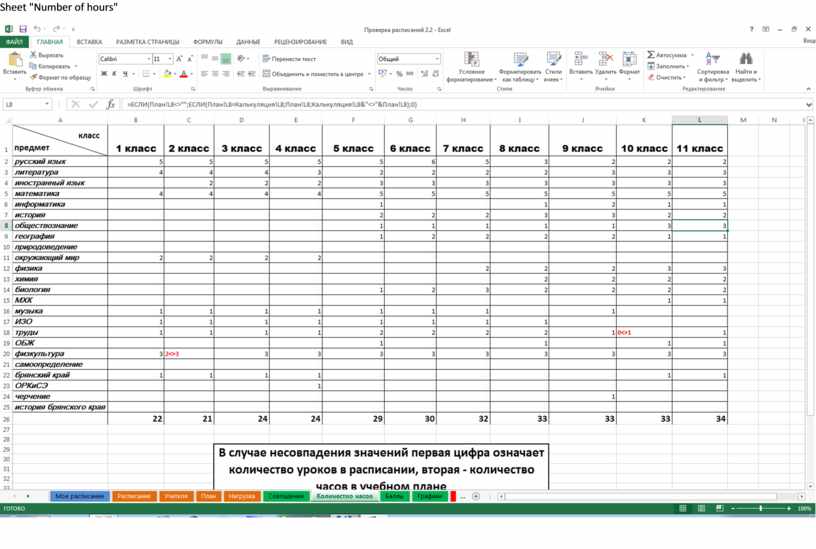
Well, now let's create a sheet "NUMBER OF HOURS" by copying the sheet "Plan". Here we will compare the indicators of the baseline plan with the obtained values. And I want the user to see what it is in case of a mismatch. Therefore, in this case, a message like "X <> Y" will be displayed, where X is the number of hours in the schedule, and Y is in the baseline. For clarity, we will also highlight this message in red.

Our task is simple - to compare the corresponding cell values ​​in the "Plan" and "Calculation" sheets using the IF function. The condition is simple (again - for cell B2) - Plan! B2 = Calculation! B2. If it is fulfilled, then simply output the Plan! B2 value.

If it is not fulfilled, then we display the following: Calculation! B2 & "<>" & Plan! B2. It seems that everything is clear here - the & symbol means concatenation of line fragments.

Again - we will check for the presence of a value in the "Plan" sheet - is there any given subject in the curriculum of this class. If not, we set the value to 0, and for greater beauty, we will also hide these zeros using the same conditional formatting. As a result, we get a ready-made formula:

= IF (Plan! B2 <> ""; IF (Plan! B2 = Calculation! B2; Plan! B2; Calculation! B2 & "<>" & Plan! B2); 0)

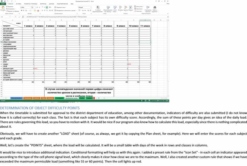
Multiplying this formula by filling horizontally and vertically, we get a finished sheet that will clearly demonstrate to us whether we have all the clocks in place.

True, there is a small nuance here - if there are subjects in the curriculum for which not a whole number of hours are allocated, then you will have to somehow contrive. For example, in the 8th and 9th grade, half an hour of music and fine arts, and we get out of the situation by recording 1 hour of music in grade 8, and 1 hour of fine art in 9th grade. Well, etc. In general, you can always find a way out. In this case, these are just such small flaws that cannot spoil the overall picture. But we have already made a full-fledged assistant for your Deputy Director for Academic Affairs!

DETERMINATION OF OBJECT DIFFICULTY POINTS

When the timetable is submitted for approval to the district department of education, among other documentation, indicators of difficulty are also submitted (I do not know how it is called correctly) for each class. The fact is that each subject has its own difficulty score. Accordingly, the sum of these points per day gives an idea of ​​the daily load. There are rules governing this load, so you have to reckon with it. It would be nice if our program also knew how to calculate this load, especially since there is nothing complicated about it.

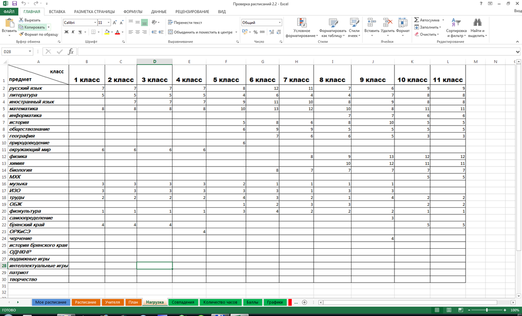
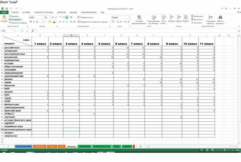
Obviously, we will have to create another "LOAD" sheet (of course, as always, we get it by copying the Plan sheet, for example). Here we will enter the scores for each subject and each grade.

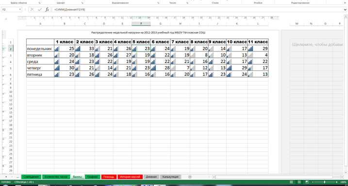
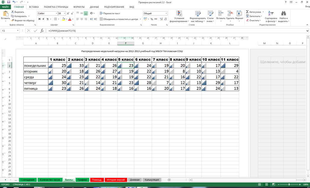
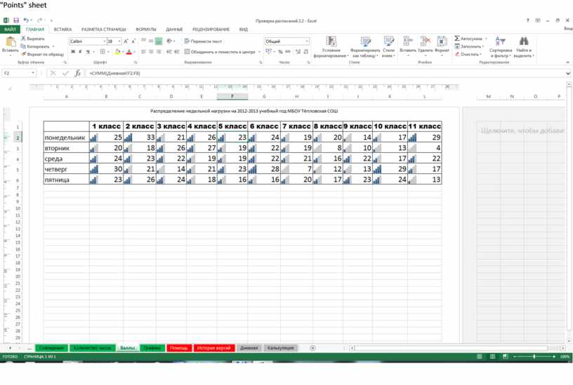
Well, let's create the "POINTS" sheet, where the load will be calculated. It will be a small table with days of the week in rows and classes in columns.

It would be nice to introduce additional indication. Conditional formatting will help us with this again. I added a preset rule from the "Icon Set" - in each cell an indicator appeared according to the type of the cell phone signal level, which clearly makes it clear how close we are to the maximum. Well, I also created another custom rule that shows if we have exceeded the maximum permissible load (something like 55 or 60 points). Then the cell lights up red.

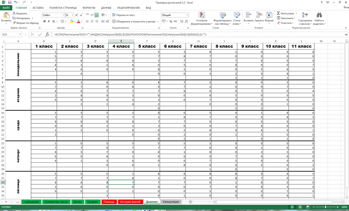
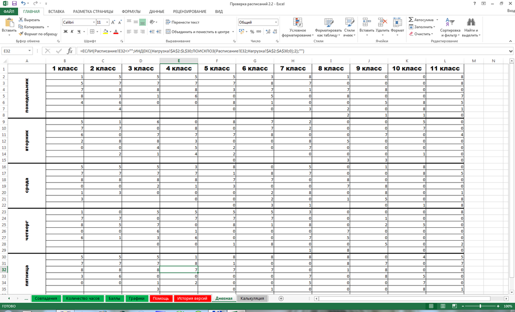
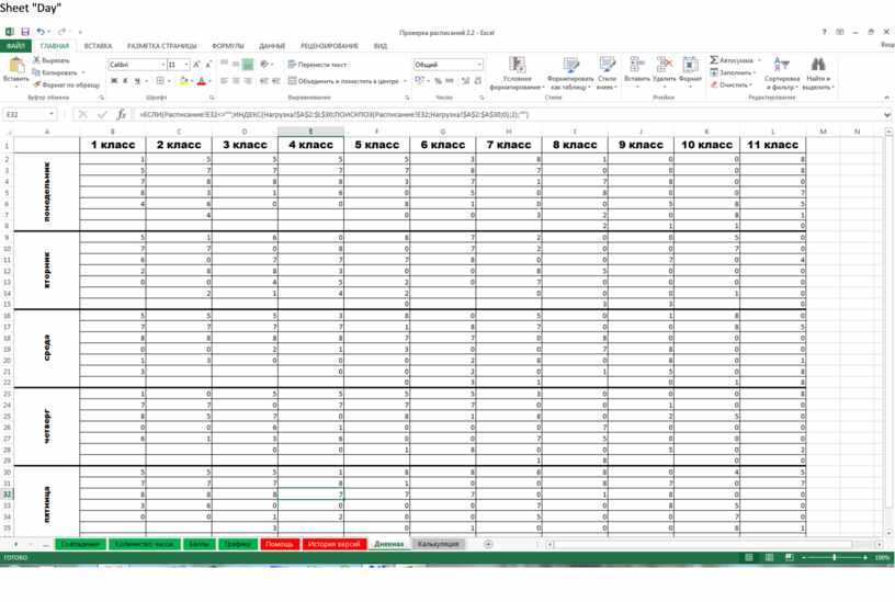
By and large, it all depends on your imagination. However, we need to get these same daily score values. Those. calculate the amount of points for each day. And to do this, we will have to create another auxiliary sheet. I called it "DAY" and got it by copying ... Well, you already understood.

On this worksheet, we have to convert the subject schedule into a points schedule. The operation is similar to what we did when converting the subject schedule into the teachers' schedule, so I see no reason to describe these actions in detail. So I'll just give the final formula for cell B2:

= IF (Schedule! B2 <> ""; INDEX (Load! $ A $ 2: $ L $ 30; SEARCH (Schedule! B2; Load! $ A $ 2: $ A $ 30; 0); 2); "")

Obviously, here we will also have to change the column number (2 in our example) to 3, 4, 5 ... depending on how we will progress to high school.

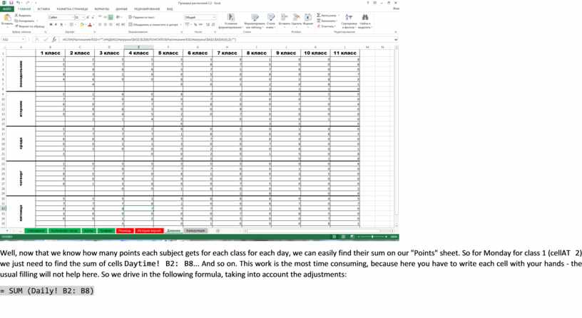
Well, now that we know how many points each subject gets for each class for each day, we can easily find their sum on our "Points" sheet. So for Monday for class 1 (cellAT 2) we just need to find the sum of cells Daytime! B2: B8... And so on. This work is the most time consuming, because here you have to write each cell with your hands - the usual filling will not help here. So we drive in the following formula, taking into account the adjustments:

= SUM (Daily! B2: B8)

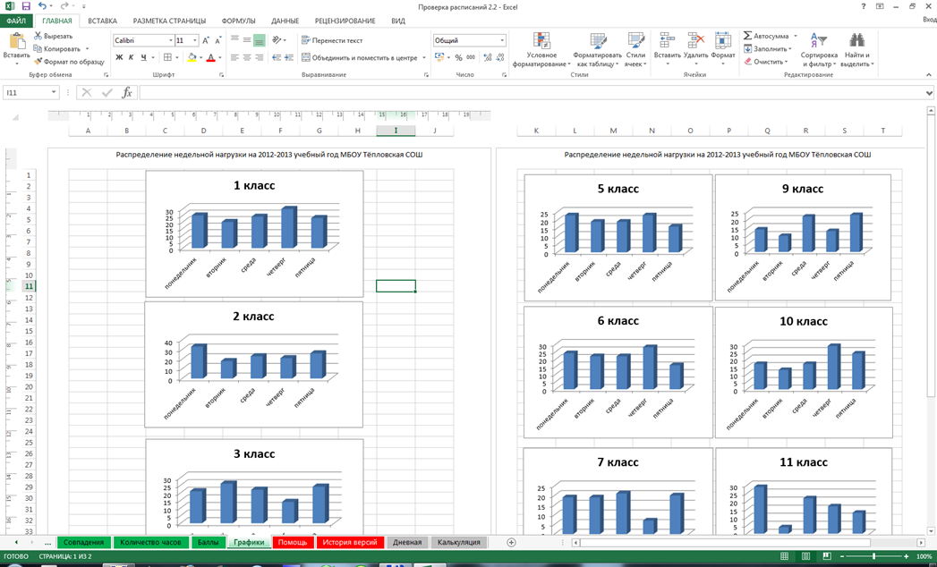
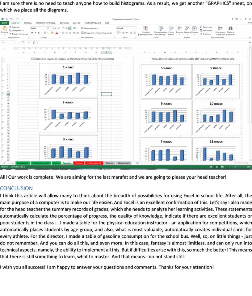
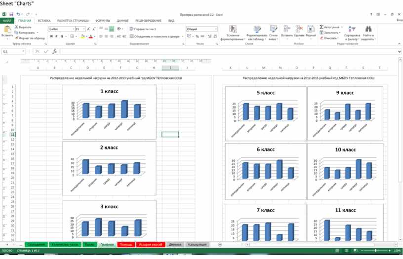
Well, the last thing - we will build weekly load schedules - they are also needed to approve the schedule in higher authorities.

I am sure there is no need to teach anyone how to build histograms. As a result, we get another "GRAPHICS" sheet, on which we place all the diagrams.

All! Our work is complete! We are aiming for the last marafet and we are going to please your head teacher!

CONCLUSION

I think this article will allow many to think about the breadth of possibilities for using Excel in school life. After all, the main purpose of a computer is to make our life easier. And Excel is an excellent confirmation of this. Let's say I also made for the head teacher the summary records of grades, which she needs to analyze her learning activities. These statements automatically calculate the percentage of progress, the quality of knowledge, indicate if there are excellent students or poor students in the class ... I made a table for the physical education instructor - an application for competitions, which automatically places students by age group, and also, what is most valuable, automatically creates individual cards for every athlete. For the director, I made a table of gasoline consumption for the school bus. Well, so, on little things - just do not remember. And you can do all this, and even more. In this case, fantasy is almost limitless, and can only run into technical aspects, namely, the ability to implement all this. But if difficulties arise with this, so much the better! This means that there is still something to learn, what to master. And that means - do not stand still.

I wish you all success! I am happy to answer your questions and comments. Thanks for your attention!

APPENDICES. SCREENSHOTS

sheet "Schedule"

"Teachers" sheet

Worksheet "Matches"

Sheet "Plan"

"Costing" sheet

Sheet "Number of hours"

Sheet "Load"

Sheet "Day"

"Points" sheet

Sheet "Charts"