Mechanical properties of the solid bodies Simulation

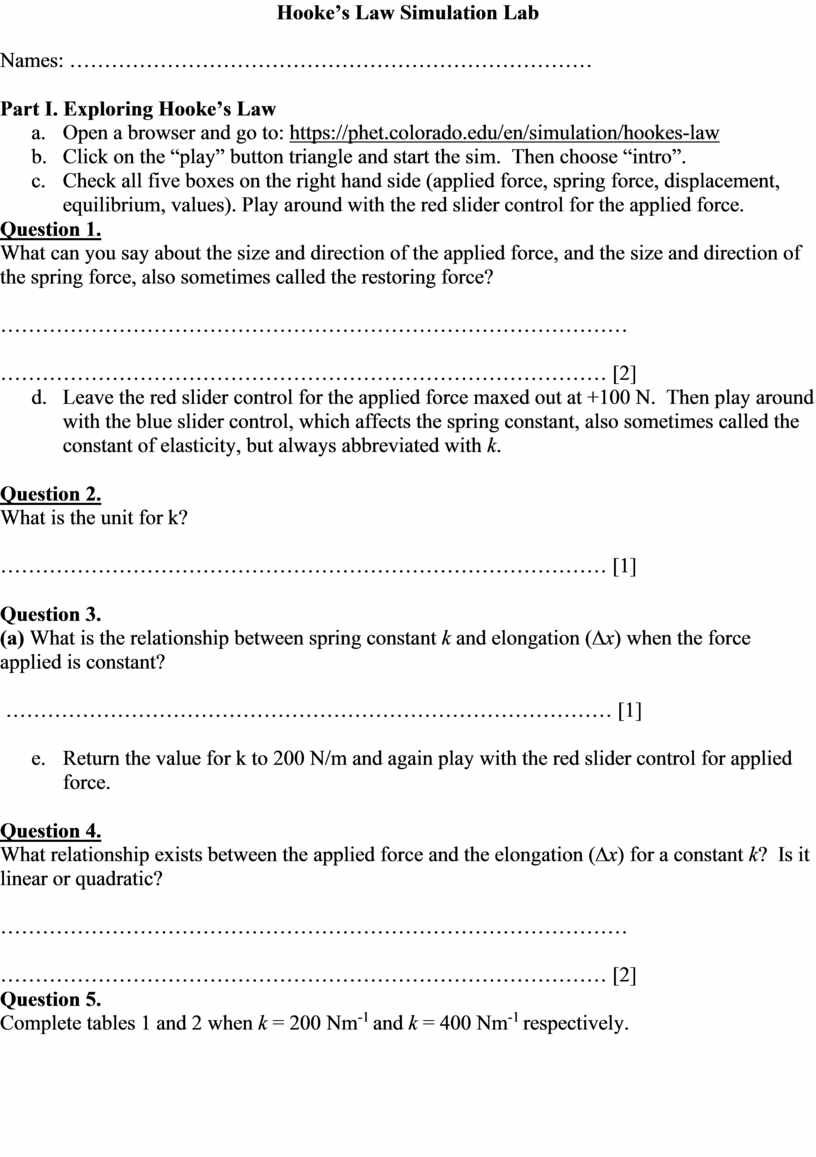
Hooke’s Law Simulation Lab

Names: …………………………………………………………………

Part I. Exploring Hooke’s Law

a.       Open a browser and go to: https://phet.colorado.edu/en/simulation/hookes-law

b.      Click on the “play” button triangle and start the sim.  Then choose “intro”.

c.       Check all five boxes on the right hand side (applied force, spring force, displacement, equilibrium, values). Play around with the red slider control for the applied force.

Question 1.

What can you say about the size and direction of the applied force, and the size and direction of the spring force, also sometimes called the restoring force?

………………………………………………………………………………

…………………………………………………………………………… [2]

d.      Leave the red slider control for the applied force maxed out at +100 N.  Then play around with the blue slider control, which affects the spring constant, also sometimes called the constant of elasticity, but always abbreviated with k.

Question 2.

What is the unit for k?

…………………………………………………………………………… [1]

Question 3.

(a) What is the relationship between spring constant k and elongation (∆x) when the force applied is constant?

 …………………………………………………………………………… [1]

e.       Return the value for k to 200 N/m and again play with the red slider control for applied force.

Question 4.

What relationship exists between the applied force and the elongation (∆x) for a constant k?  Is it linear or quadratic?

………………………………………………………………………………

…………………………………………………………………………… [2]

Question 5.

Complete tables 1 and 2 when k = 200 Nm^-1 and k = 400 Nm^-1 respectively.

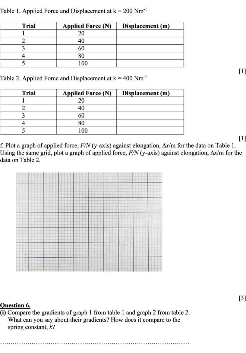
Table 1. Applied Force and Displacement at k = 200 Nm^-1

[1]

Table 2. Applied Force and Displacement at k = 400 Nm^-1

[1]

f. Plot a graph of applied force, F/N (y-axis) against elongation, ∆x/m for the data on Table 1. Using the same grid, plot a graph of applied force, F/N (y-axis) against elongation, ∆x/m for the data on Table 2.

[3]

Question 6.

(i) Compare the gradients of graph 1 from table 1 and graph 2 from table 2.

     What can you say about their gradients? How does it compare to the    

     spring constant, k?

………………………………………………………………………………

…………………………………………………………………………… [2]

(ii)  What can you conclude about the gradient of F against ∆x and spring constant?

………………………………………………………………………………

…………………………………………………………………………… [1]

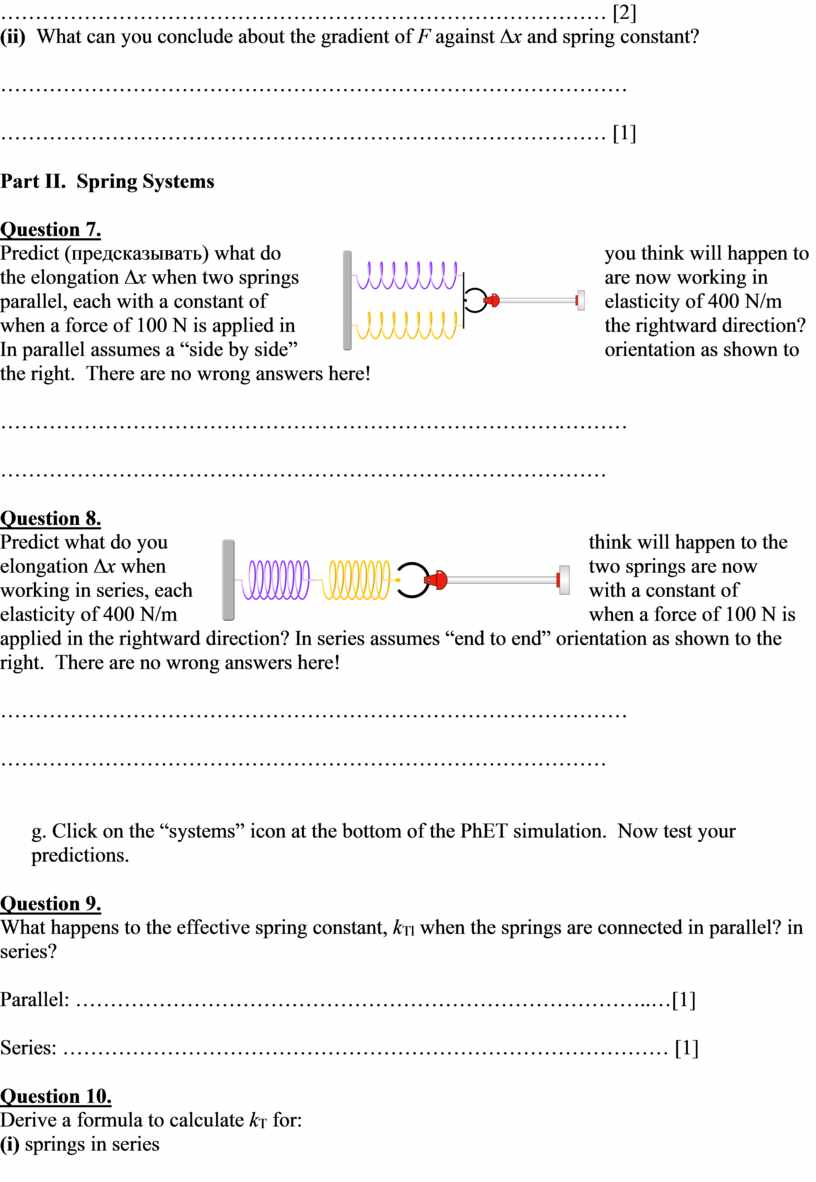
Part II.  Spring Systems

Question 7.

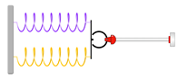Predict (предсказывать) what do you think will happen to the elongation ∆x when two springs are now working in parallel, each with a constant of elasticity of 400 N/m when a force of 100 N is applied in the rightward direction? In parallel assumes a “side by side” orientation as shown to the right.  There are no wrong answers here!

………………………………………………………………………………

……………………………………………………………………………

Question 8.

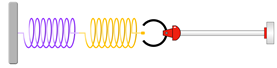Predict what do you think will happen to the elongation ∆x when two springs are now working in series, each with a constant of elasticity of 400 N/m when a force of 100 N is applied in the rightward direction? In series assumes “end to end” orientation as shown to the right.  There are no wrong answers here!

………………………………………………………………………………

……………………………………………………………………………

g. Click on the “systems” icon at the bottom of the PhET simulation.  Now test your predictions.

Question 9.

What happens to the effective spring constant, k_Tl when the springs are connected in parallel? in series?

Parallel: ………………………………………………………………………..…[1]

Series: …………………………………………………………………………… [1]

Question 10.

Derive a formula to calculate k_T for:

(i) springs in series

[2]

(ii) springs in parallel

[2]

Скачано с www.znanio.ru