didactics (19)

Shortest path algorithm on graph implementation theory

Twitter Example: Tweet Delivery Problem

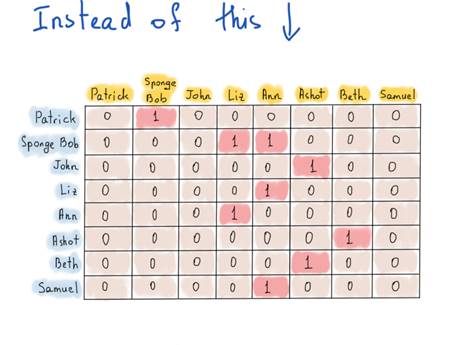
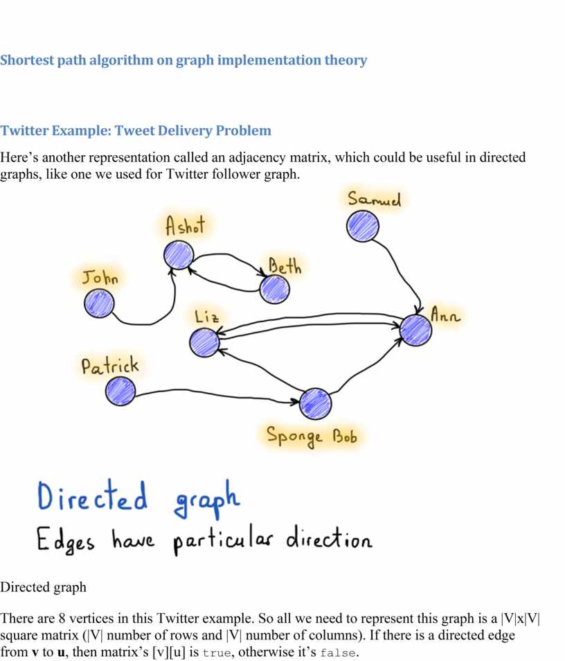
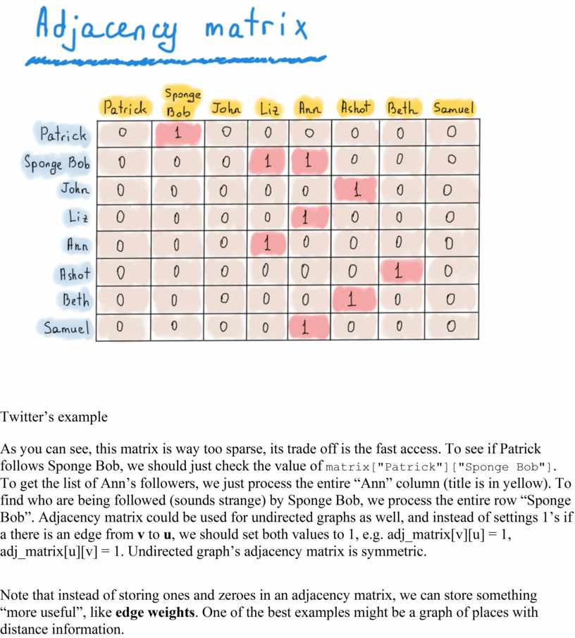
Here’s another representation called an adjacency matrix, which could be useful in directed graphs, like one we used for Twitter follower graph.

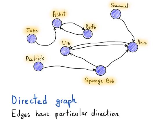
Directed graph

There are 8 vertices in this Twitter example. So all we need to represent this graph is a |V|x|V| square matrix (|V| number of rows and |V| number of columns). If there is a directed edge from v to u, then matrix’s [v][u] is true, otherwise it’s false.

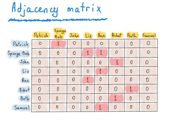
Twitter’s example

As you can see, this matrix is way too sparse, its trade off is the fast access. To see if Patrick follows Sponge Bob, we should just check the value of matrix["Patrick"]["Sponge Bob"]. To get the list of Ann’s followers, we just process the entire “Ann” column (title is in yellow). To find who are being followed (sounds strange) by Sponge Bob, we process the entire row “Sponge Bob”. Adjacency matrix could be used for undirected graphs as well, and instead of settings 1’s if a there is an edge from v to u, we should set both values to 1, e.g. adj_matrix[v][u] = 1, adj_matrix[u][v] = 1. Undirected graph’s adjacency matrix is symmetric.

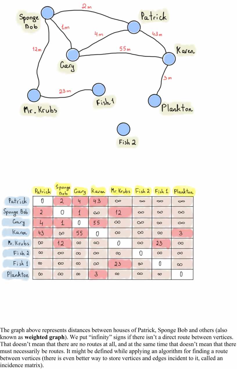
Note that instead of storing ones and zeroes in an adjacency matrix, we can store something “more useful”, like edge weights. One of the best examples might be a graph of places with distance information.

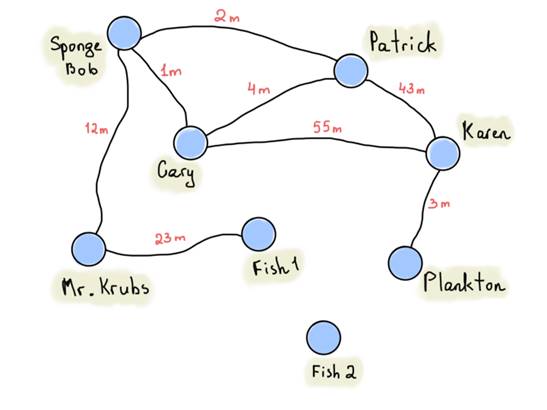
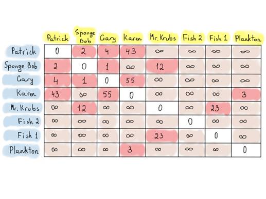
The graph above represents distances between houses of Patrick, Sponge Bob and others (also known as weighted graph). We put “infinity” signs if there isn’t a direct route between vertices. That doesn’t mean that there are no routes at all, and at the same time that doesn’t mean that there must necessarily be routes. It might be defined while applying an algorithm for finding a route between vertices (there is even better way to store vertices and edges incident to it, called an incidence matrix).

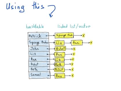
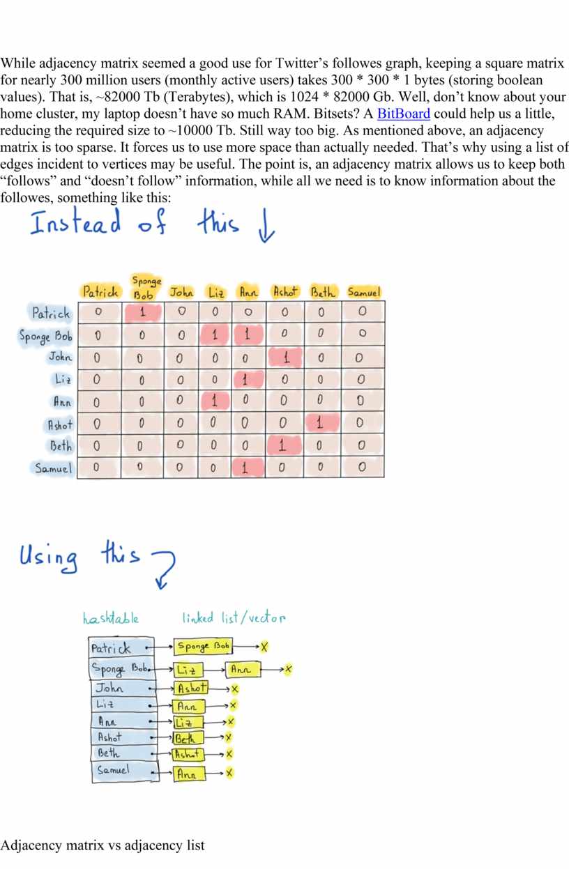
While adjacency matrix seemed a good use for Twitter’s followes graph, keeping a square matrix for nearly 300 million users (monthly active users) takes 300 * 300 * 1 bytes (storing boolean values). That is, ~82000 Tb (Terabytes), which is 1024 * 82000 Gb. Well, don’t know about your home cluster, my laptop doesn’t have so much RAM. Bitsets? A BitBoard could help us a little, reducing the required size to ~10000 Tb. Still way too big. As mentioned above, an adjacency matrix is too sparse. It forces us to use more space than actually needed. That’s why using a list of edges incident to vertices may be useful. The point is, an adjacency matrix allows us to keep both “follows” and “doesn’t follow” information, while all we need is to know information about the followes, something like this:

Adjacency matrix vs adjacency list

The illustration at the right side is called an adjacency list. Each list describes the set of neighbors of a vertex in the graph. By the way, the actual implementation of the graph representation as an adjacency list, again, differs (ridiculous facts). In the illustration, we highlighted a hashtable usage, which is reasonable, as the access of any vertex will be O(1), and for the list of neighbor vertices we didn’t mention the exact data structure, deviating from linked lists to vectors. Choice is yours.

Traversals: DFS and BFS

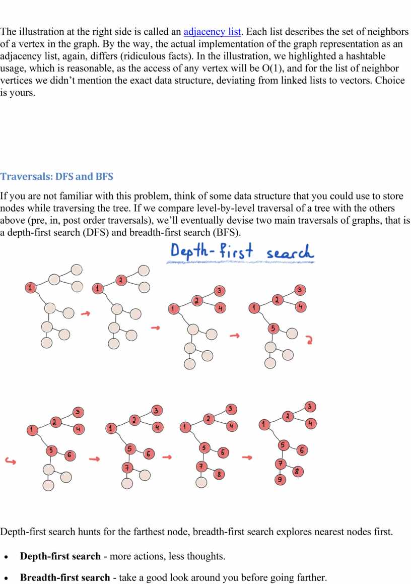
If you are not familiar with this problem, think of some data structure that you could use to store nodes while traversing the tree. If we compare level-by-level traversal of a tree with the others above (pre, in, post order traversals), we’ll eventually devise two main traversals of graphs, that is a depth-first search (DFS) and breadth-first search (BFS).

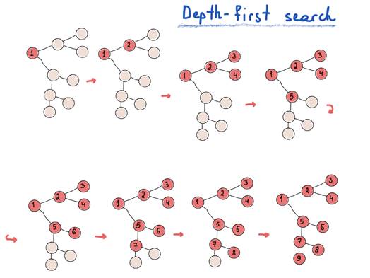
Depth-first search hunts for the farthest node, breadth-first search explores nearest nodes first.

·         Depth-first search - more actions, less thoughts.

·         Breadth-first search - take a good look around you before going farther.

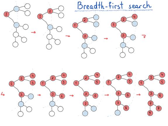
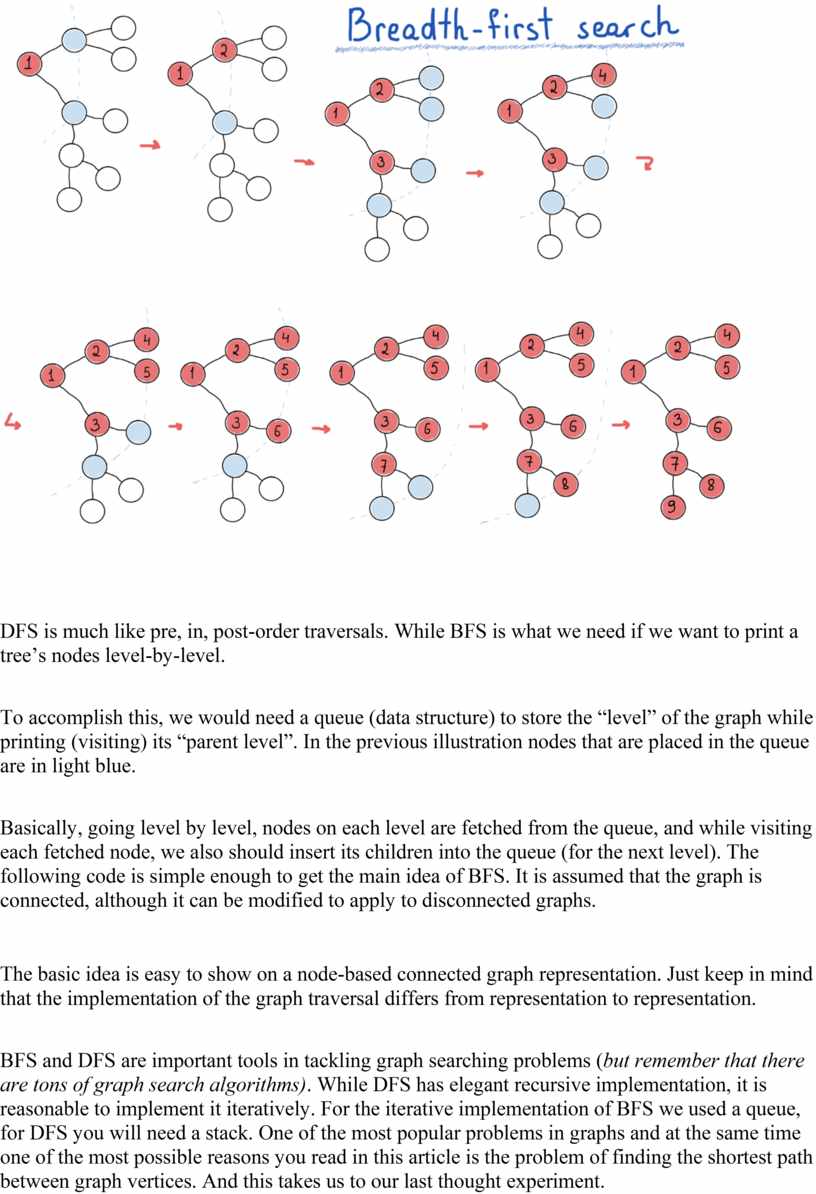
DFS is much like pre, in, post-order traversals. While BFS is what we need if we want to print a tree’s nodes level-by-level.

To accomplish this, we would need a queue (data structure) to store the “level” of the graph while printing (visiting) its “parent level”. In the previous illustration nodes that are placed in the queue are in light blue.

Basically, going level by level, nodes on each level are fetched from the queue, and while visiting each fetched node, we also should insert its children into the queue (for the next level). The following code is simple enough to get the main idea of BFS. It is assumed that the graph is connected, although it can be modified to apply to disconnected graphs.

The basic idea is easy to show on a node-based connected graph representation. Just keep in mind that the implementation of the graph traversal differs from representation to representation.

BFS and DFS are important tools in tackling graph searching problems (but remember that there are tons of graph search algorithms). While DFS has elegant recursive implementation, it is reasonable to implement it iteratively. For the iterative implementation of BFS we used a queue, for DFS you will need a stack. One of the most popular problems in graphs and at the same time one of the most possible reasons you read in this article is the problem of finding the shortest path between graph vertices. And this takes us to our last thought experiment.

Uber and the Shortest Path Problem (Dijkstra’s Algorithm)

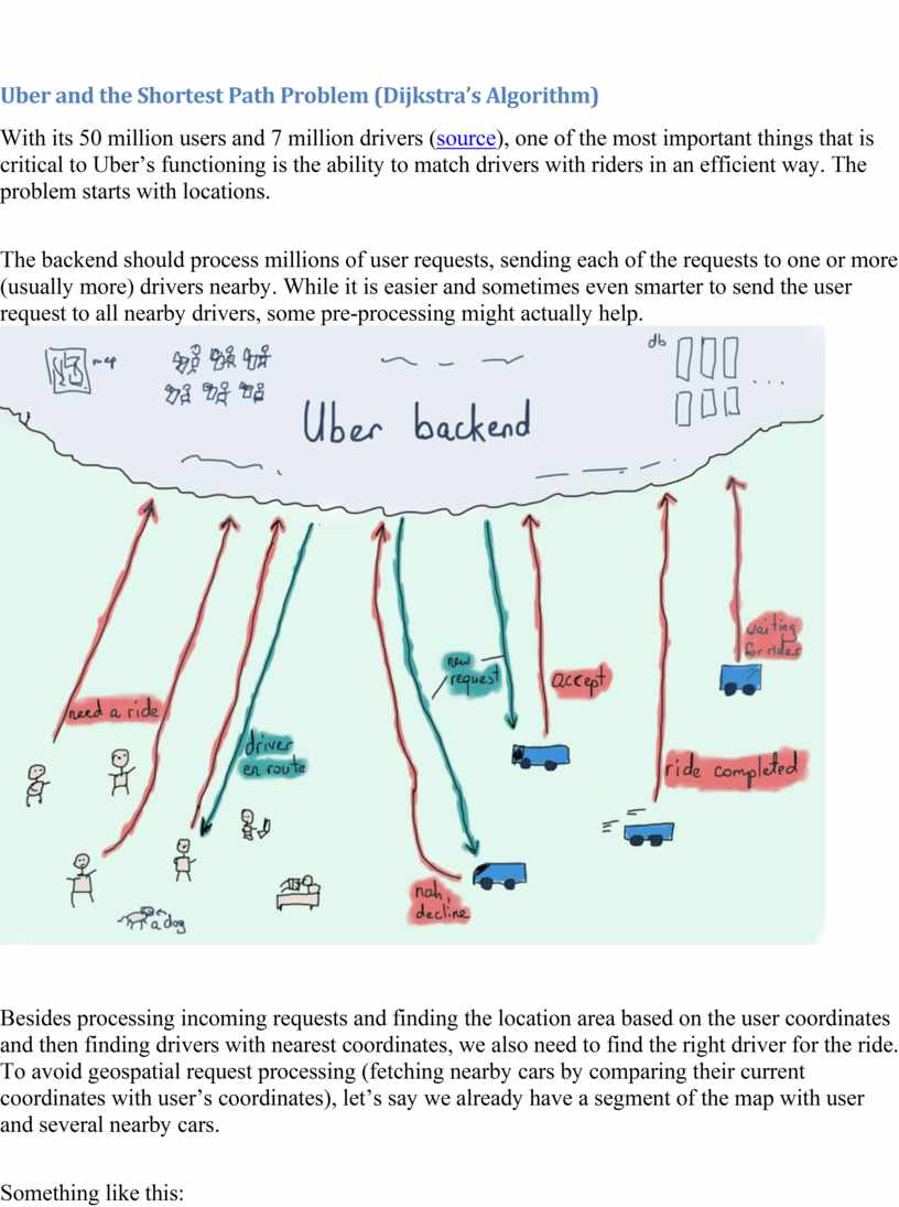
With its 50 million users and 7 million drivers (source), one of the most important things that is critical to Uber’s functioning is the ability to match drivers with riders in an efficient way. The problem starts with locations.

The backend should process millions of user requests, sending each of the requests to one or more (usually more) drivers nearby. While it is easier and sometimes even smarter to send the user request to all nearby drivers, some pre-processing might actually help.

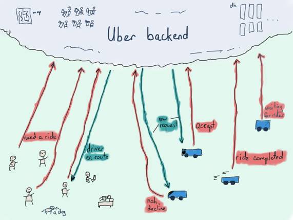
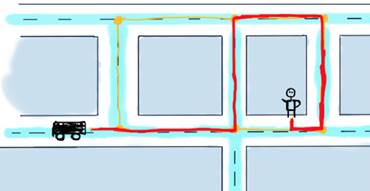
Besides processing incoming requests and finding the location area based on the user coordinates and then finding drivers with nearest coordinates, we also need to find the right driver for the ride. To avoid geospatial request processing (fetching nearby cars by comparing their current coordinates with user’s coordinates), let’s say we already have a segment of the map with user and several nearby cars.

Something like this:

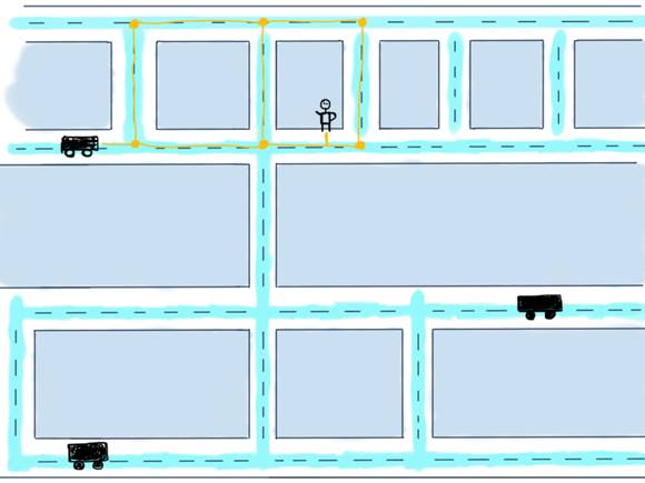
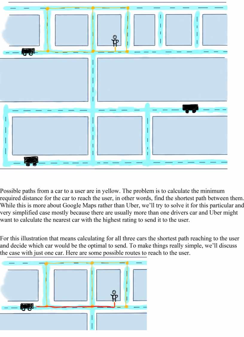
Possible paths from a car to a user are in yellow. The problem is to calculate the minimum required distance for the car to reach the user, in other words, find the shortest path between them. While this is more about Google Maps rather than Uber, we’ll try to solve it for this particular and very simplified case mostly because there are usually more than one drivers car and Uber might want to calculate the nearest car with the highest rating to send it to the user.

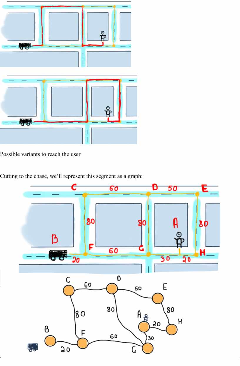
For this illustration that means calculating for all three cars the shortest path reaching to the user and decide which car would be the optimal to send. To make things really simple, we’ll discuss the case with just one car. Here are some possible routes to reach to the user.

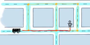
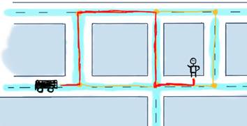
Possible variants to reach the user

Cutting to the chase, we’ll represent this segment as a graph:

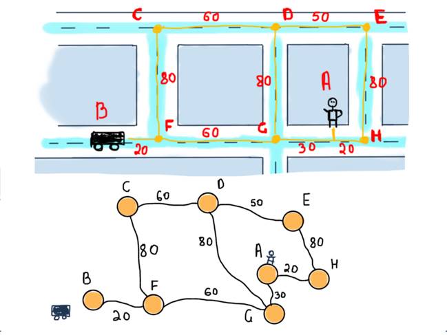
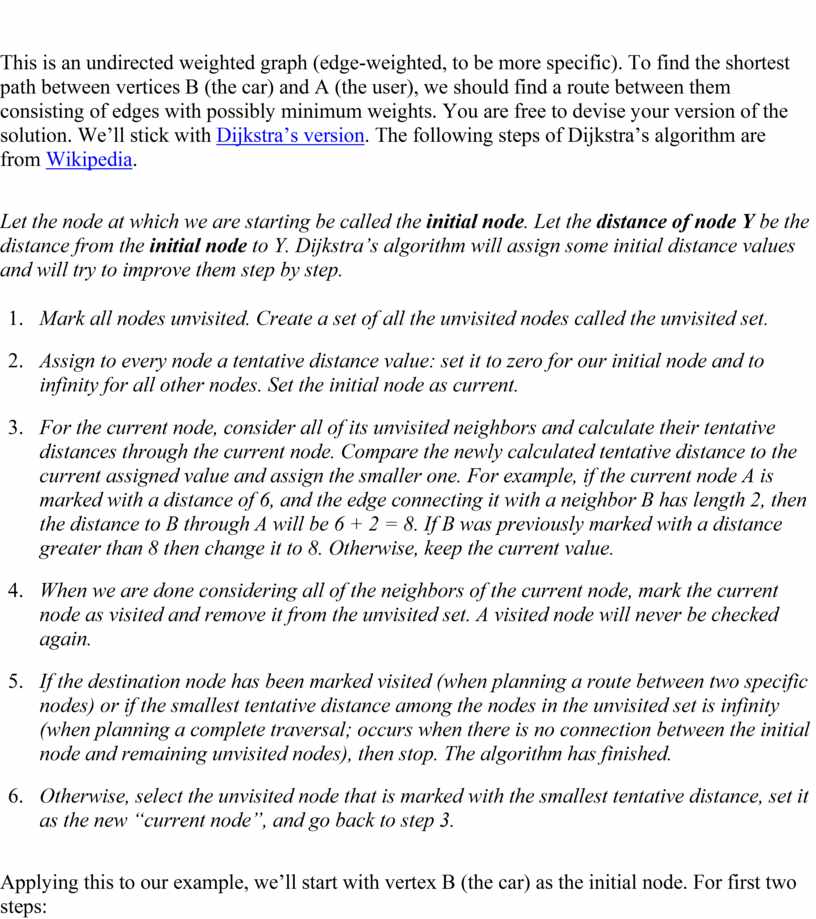
This is an undirected weighted graph (edge-weighted, to be more specific). To find the shortest path between vertices B (the car) and A (the user), we should find a route between them consisting of edges with possibly minimum weights. You are free to devise your version of the solution. We’ll stick with Dijkstra’s version. The following steps of Dijkstra’s algorithm are from Wikipedia.

Let the node at which we are starting be called the initial node. Let the distance of node Y be the distance from the initial node to Y. Dijkstra’s algorithm will assign some initial distance values and will try to improve them step by step.

1.      Mark all nodes unvisited. Create a set of all the unvisited nodes called the unvisited set.

2.      Assign to every node a tentative distance value: set it to zero for our initial node and to infinity for all other nodes. Set the initial node as current.

3.      For the current node, consider all of its unvisited neighbors and calculate their tentative distances through the current node. Compare the newly calculated tentative distance to the current assigned value and assign the smaller one. For example, if the current node A is marked with a distance of 6, and the edge connecting it with a neighbor B has length 2, then the distance to B through A will be 6 + 2 = 8. If B was previously marked with a distance greater than 8 then change it to 8. Otherwise, keep the current value.

4.      When we are done considering all of the neighbors of the current node, mark the current node as visited and remove it from the unvisited set. A visited node will never be checked again.

5.      If the destination node has been marked visited (when planning a route between two specific nodes) or if the smallest tentative distance among the nodes in the unvisited set is infinity (when planning a complete traversal; occurs when there is no connection between the initial node and remaining unvisited nodes), then stop. The algorithm has finished.

6.      Otherwise, select the unvisited node that is marked with the smallest tentative distance, set it as the new “current node”, and go back to step 3.

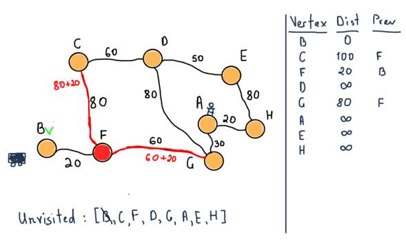
Applying this to our example, we’ll start with vertex B (the car) as the initial node. For first two steps:

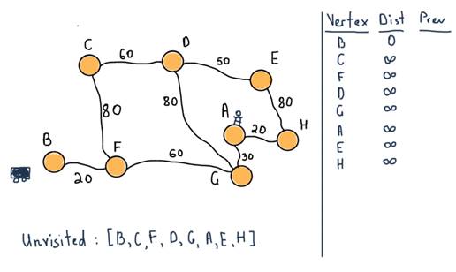
Our unvisited set consists of all vertices. Also note the table at the left side of the illustration. For all vertices, it will contain all the shortest distances from B and the previous (marked “Prev”) vertex that lead to the vertex. For instance the distance is 20 from B to F, and the previous vertex is B.

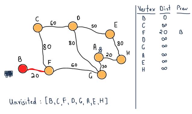
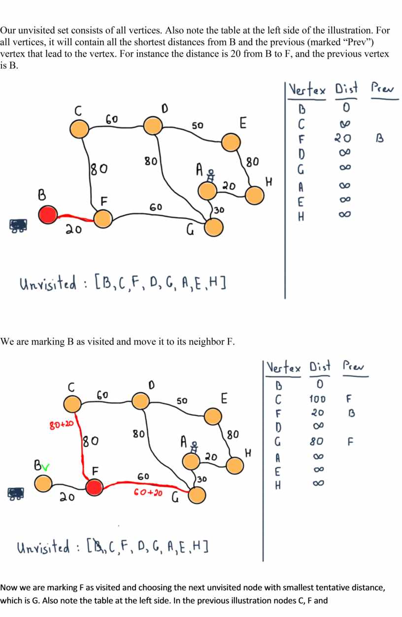
We are marking B as visited and move it to its neighbor F.

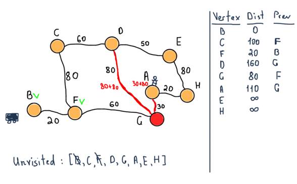
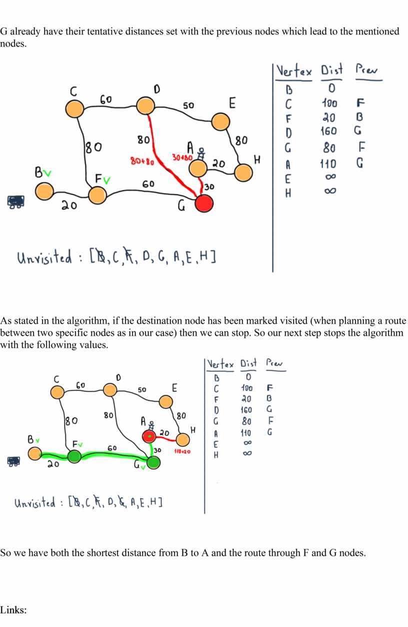
Now we are marking F as visited and choosing the next unvisited node with smallest tentative distance, which is G. Also note the table at the left side. In the previous illustration nodes C, F and G already have their tentative distances set with the previous nodes which lead to the mentioned nodes.

As stated in the algorithm, if the destination node has been marked visited (when planning a route between two specific nodes as in our case) then we can stop. So our next step stops the algorithm with the following values.

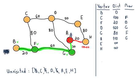
So we have both the shortest distance from B to A and the route through F and G nodes.

Links:

https://medium.freecodecamp.org/i-dont-understand-graph-theory-1c96572a1401

Скачано с www.znanio.ru