methodological_instructions (19)

Methodological Instructions

Theme: Algorithms on graphs 

Aim: Implementation of search algorithms on graphs to solve the practical tasks

Lesson objective: Study directed graph and shortest path algorithm

Assessment criteria

Knowledge

·     Know what the directed graph is

Comprehension

·     Describe Depth First Search

·     Describe Breadth First Search

• Describe the shortest path algorithm

Language objectives

Learners able to …

• State what are Depth First Search and Breadth First Search

• Describe the search process in shortest path algorithm

Vocabulary and terminology specific to the subject:

Adjacency matrix, adjacency list,  initial node, path, root, vertices, edge, weighted graph

Useful expressions for dialogs and letters:

Well, Depth First Search follows to this logic: … .

For example, directed graph illustrates not only the connections between …. .

Obviously, finding the shortest path between initial node and ….

Theory

Traversals: DFS and BFS

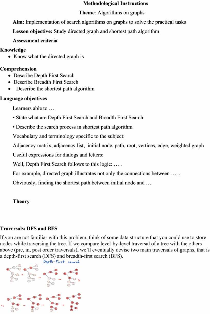
If you are not familiar with this problem, think of some data structure that you could use to store nodes while traversing the tree. If we compare level-by-level traversal of a tree with the others above (pre, in, post order traversals), we’ll eventually devise two main traversals of graphs, that is a depth-first search (DFS) and breadth-first search (BFS).

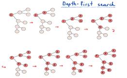
Depth-first search hunts for the farthest node, breadth-first search explores nearest nodes first.

·                  Depth-first search - more actions, less thoughts.

·                  Breadth-first search - take a good look around you before going farther.

·         DFS is much like pre, in, post-order traversals. While BFS is what we need if we want to print a tree’s nodes level-by-level.

·         To accomplish this, we would need a queue (data structure) to store the “level” of the graph while printing (visiting) its “parent level”. In the previous illustration nodes that are placed in the queue are in light blue.

·         Basically, going level by level, nodes on each level are fetched from the queue, and while visiting each fetched node, we also should insert its children into the queue (for the next level). The following code is simple enough to get the main idea of BFS. It is assumed that the graph is connected, although it can be modified to apply to disconnected graphs.

·         The basic idea is easy to show on a node-based connected graph representation. Just keep in mind that the implementation of the graph traversal differs from representation to representation.

·         BFS and DFS are important tools in tackling graph searching problems (but remember that there are tons of graph search algorithms). While DFS has elegant recursive implementation, it is reasonable to implement it iteratively. For the iterative implementation of BFS we used a queue, for DFS you will need a stack. One of the most popular problems in graphs and at the same time one of the most possible reasons you read in this article is the problem of finding the shortest path between graph vertices. And this takes us to our last thought experiment.

·         Uber and the Shortest Path Problem (Dijkstra’s Algorithm)

·         With its 50 million users and 7 million drivers (source), one of the most important things that is critical to Uber’s functioning is the ability to match drivers with riders in an efficient way. The problem starts with locations.

·         The backend should process millions of user requests, sending each of the requests to one or more (usually more) drivers nearby. While it is easier and sometimes even smarter to send the user request to all nearby drivers, some pre-processing might actually help.

Let the node at which we are starting be called the initial node. Let the distance of node Y be the distance from the initial node to Y. Dijkstra’s algorithm will assign some initial distance values and will try to improve them step by step.

1.               Mark all nodes unvisited. Create a set of all the unvisited nodes called the unvisited set.

2.               Assign to every node a tentative distance value: set it to zero for our initial node and to infinity for all other nodes. Set the initial node as current.

3.               For the current node, consider all of its unvisited neighbors and calculate their tentative distances through the current node. Compare the newly calculated tentative distance to the current assigned value and assign the smaller one. For example, if the current node A is marked with a distance of 6, and the edge connecting it with a neighbor B has length 2, then the distance to B through A will be 6 + 2 = 8. If B was previously marked with a distance greater than 8 then change it to 8. Otherwise, keep the current value.

4.               When we are done considering all of the neighbors of the current node, mark the current node as visited and remove it from the unvisited set. A visited node will never be checked again.

5.               If the destination node has been marked visited (when planning a route between two specific nodes) or if the smallest tentative distance among the nodes in the unvisited set is infinity (when planning a complete traversal; occurs when there is no connection between the initial node and remaining unvisited nodes), then stop. The algorithm has finished.

6.               Otherwise, select the unvisited node that is marked with the smallest tentative distance, set it as the new “current node”, and go back to step 3.

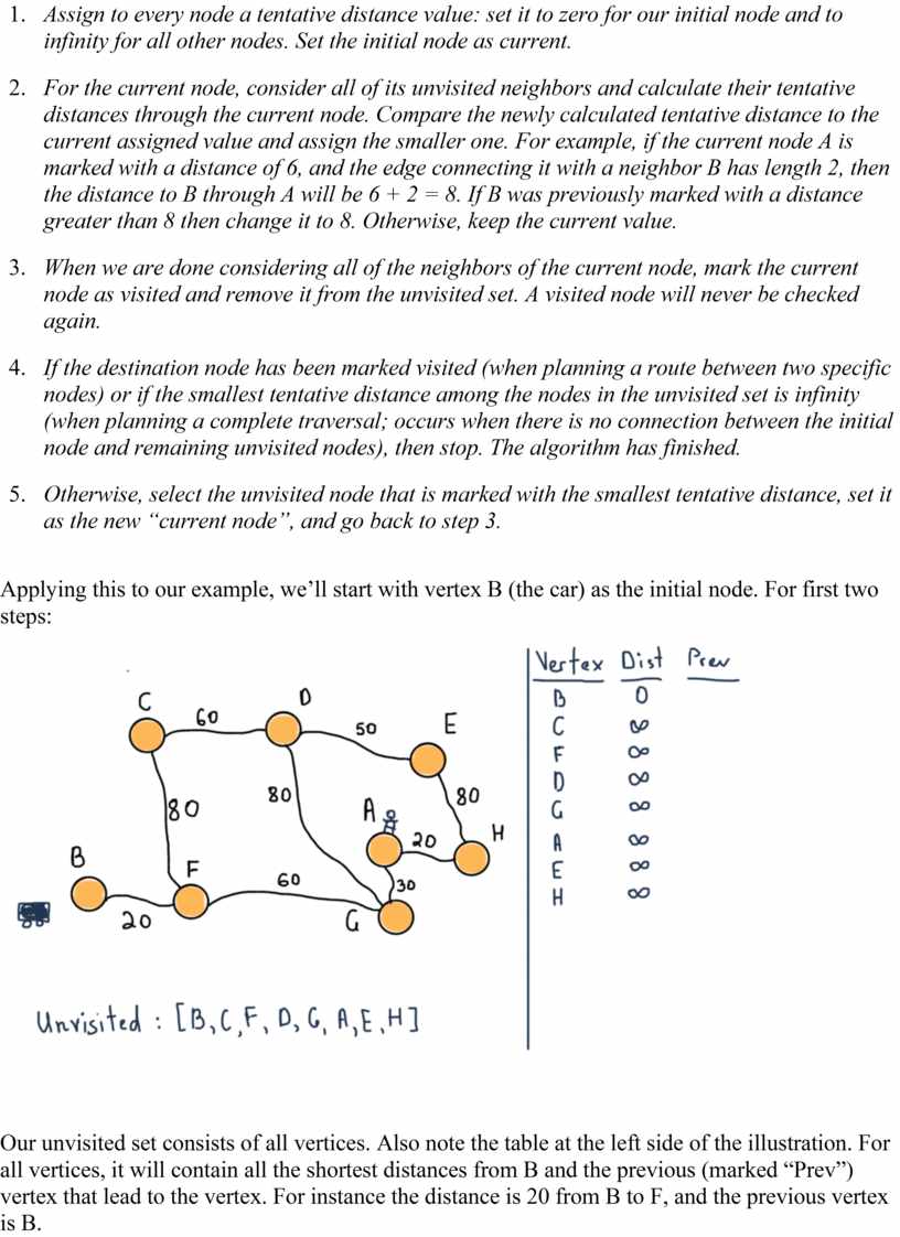
Applying this to our example, we’ll start with vertex B (the car) as the initial node. For first two steps:

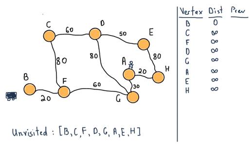
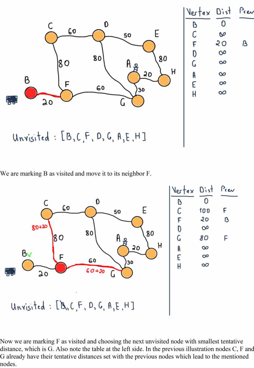
Our unvisited set consists of all vertices. Also note the table at the left side of the illustration. For all vertices, it will contain all the shortest distances from B and the previous (marked “Prev”) vertex that lead to the vertex. For instance the distance is 20 from B to F, and the previous vertex is B.

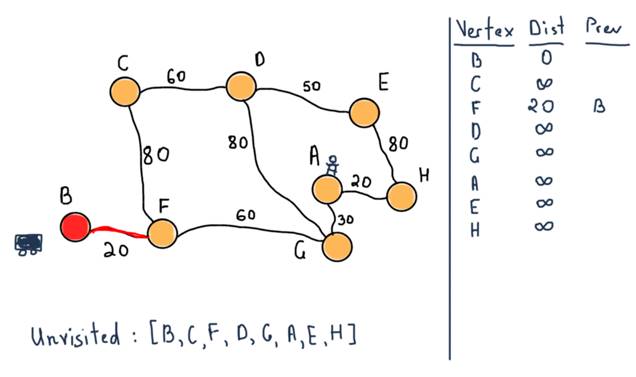
We are marking B as visited and move it to its neighbor F.

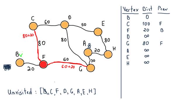
Now we are marking F as visited and choosing the next unvisited node with smallest tentative distance, which is G. Also note the table at the left side. In the previous illustration nodes C, F and G already have their tentative distances set with the previous nodes which lead to the mentioned nodes.

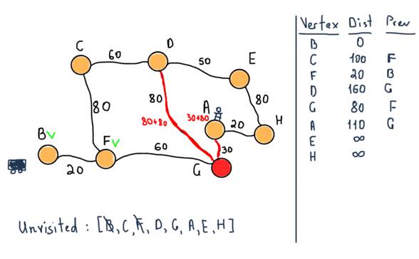
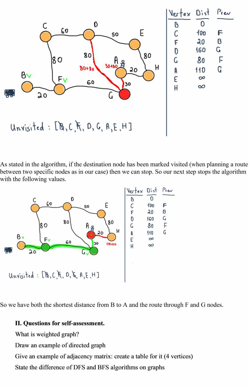
As stated in the algorithm, if the destination node has been marked visited (when planning a route between two specific nodes as in our case) then we can stop. So our next step stops the algorithm with the following values.

So we have both the shortest distance from B to A and the route through F and G nodes.

П. Questions for self-assessment.

What is weighted graph?

Draw an example of directed graph

Give an example of adjacency matrix: create a table for it (4 vertices)

State the difference of DFS and BFS algorithms on graphs

Visual Aids and Materials links.

1. Slides

2.      https://www.c-sharpcorner.com/UploadFile/19b1bd/binarysearchtreewalkstraversal-implementation-using-C-Sharp/

3.      https://en.wikibooks.org/wiki/A-level_Computing_2009/AQA/Problem_Solving,_Programming,_Operating_Systems,_Databases_and_Networking/Programming_Concepts/Tree_traversal_algorithms_for_a_binary_tree

4. https://medium.freecodecamp.org/i-dont-understand-graph-theory-1c96572a1401

Students' Practical Activities:

Students must be able:

• Describe the shortest path algorithm implementation

Скачано с www.znanio.ru